The analysis of LOS (Line of Sight) in telecommunications is the study that determines whether a clear, unobstructed path exists between a transmitting antenna and a receiver. While this calculation was traditionally reserved for large microwave links over long distances or in rural environments, the arrival of 5G networks and the horizon of 6G have turned it into an absolute priority for urban deployment, completely transforming how networks are planned in major cities.
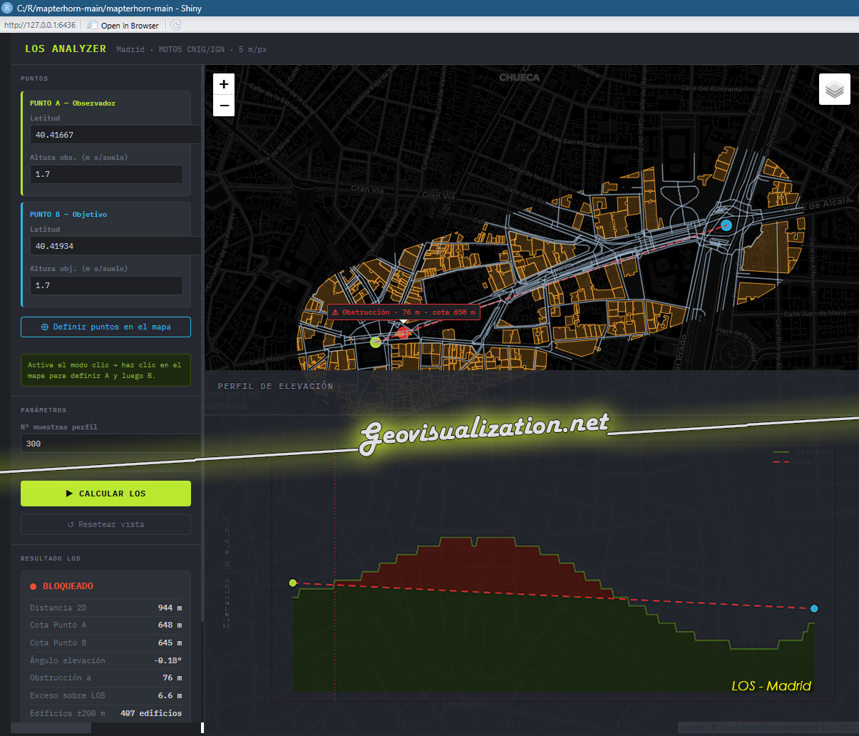
This radical shift is due to the nature of the high frequencies used by next-generation technologies, particularly millimeter waves. Unlike older 4G networks, which operated on bands capable of bending around buildings and penetrating walls with relative ease, these new frequencies offer massive speeds but behave in an almost optical manner, similar to the beam of a laser pointer. Any physical obstacle, no matter how small, completely absorbs or blocks the signal. This forces the industry to shift away from a model of large antennas on rooftops toward a hyper-dense network of micro-antennas distributed at street level on elements like lampposts, traffic lights, or bus shelters.
To map this dense urban mesh in central Madrid, telecommunications engineers rely heavily on geographic information systems and open data, where the Centro Nacional de Información Geográfica (CNIG) plays a crucial role. CNIG offers high-resolution Digital Terrain Models (5m in this case) and LiDAR flights that replicate every building and tree in the capital down to the centimeter. A key factor for the telecommunications industry is that CNIG operates under an open data license that explicitly permits commercial use. This legal framework gives operators and tech companies the absolute freedom to integrate these government-funded geographical datasets into their commercial simulation software and network planning pipelines without legal friction, significantly reducing the cost and accelerating the deployment of new infrastructure.
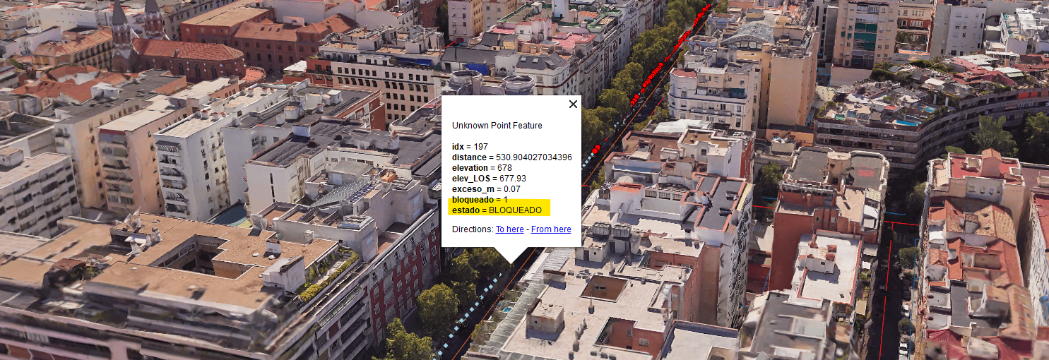
To bridge the gap between these massive raw geographic datasets and practical engineering solutions, the industry relies on specialized open-source tools, where Mapterhorn stands out as an essential link. Mapterhorn acts as a powerful bridge between R—the statistical and data computing language—and spatial data, allowing engineers to ingest, clean, and manipulate heavy LiDAR files and raster data with high performance. Through this integration, data analysts can programmatically automate the extraction of urban profiles and line-of-sight paths directly within their data pipelines.
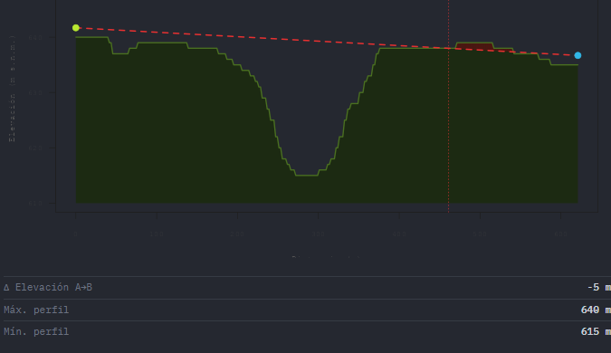
This synergy between CNIG’s open commercial-ready data and the processing capabilities of Matterhorn within the R ecosystem enables the calculation of thousands of simultaneous ray-tracing simulations. It allows engineers to predict exactly how the signal will bounce off a glass facade on Gran Vía or diffract around a narrow street corner, making the connectivity of the future viable and stable at street level, despite the architectural difficulties of central Madrid.
Please let me know if this likes you!
# Desarrollado por Alberto Concejal / Geovisualization.net# LOS Analyzer — Madrid | MDT05 IGN/CNIG via WCS# Dependencias: shiny, terra, leaflet, sf# install.packages(c("shiny","terra","leaflet","sf"))library(shiny)library(terra)library(leaflet)library(sf)library(jsonlite)# ─────────────────────────────────────────────────────────────────────────────# FUNCIONES AUXILIARES# ─────────────────────────────────────────────────────────────────────────────#' Descarga MDT05 del IGN via WCS 1.0.0 para un bounding box dado (EPSG:4326)#' Devuelve un SpatRaster en EPSG:25830 (UTM30) — sin reproyectar para evitar#' conflicto con proj.db de PostgreSQL/PostGISdescargar_mdt05 <- function(lon_min, lat_min, lon_max, lat_max, buffer_deg = 0.005) { # Buffer en grados xmin <- lon_min - buffer_deg ymin <- lat_min - buffer_deg xmax <- lon_max + buffer_deg ymax <- lat_max + buffer_deg # Convertir bbox a UTM30 via sf (sf usa su propia PROJ, funciona bien) bbox_geo <- st_bbox(c(xmin = xmin, ymin = ymin, xmax = xmax, ymax = ymax), crs = 4326) bbox_utm <- st_bbox(st_transform(st_as_sfc(bbox_geo), 25830)) # Resolución MDT05: 5 m/pixel — limitar a 800px máx res_m <- 5 width_px <- min(ceiling((bbox_utm["xmax"] - bbox_utm["xmin"]) / res_m), 800) height_px <- min(ceiling((bbox_utm["ymax"] - bbox_utm["ymin"]) / res_m), 800) url <- paste0( "https://servicios.idee.es/wcs-inspire/mdt", "?SERVICE=WCS&VERSION=1.0.0&REQUEST=GetCoverage", "&COVERAGE=Elevacion25830_5", "&CRS=EPSG:25830", "&BBOX=", bbox_utm["xmin"], ",", bbox_utm["ymin"], ",", bbox_utm["xmax"], ",", bbox_utm["ymax"], "&WIDTH=", width_px, "&HEIGHT=", height_px, "&FORMAT=GEOTIFFINT16" ) tmp <- tempfile(fileext = ".tif") tryCatch( download.file(url, tmp, mode = "wb", quiet = TRUE), error = function(e) stop("Error descargando MDT05: ", conditionMessage(e)) ) # Verificar que no es un XML de error first_line <- readLines(tmp, n = 1, warn = FALSE) if (grepl("xml|ServiceException", first_line, ignore.case = TRUE)) { stop("El WCS devolvió un error: ", paste(readLines(tmp), collapse = " ")) } r <- tryCatch( rast(tmp), error = function(e) stop("Error leyendo GeoTIFF del WCS: ", conditionMessage(e)) ) # Asignar extensión UTM30 manualmente (el WCS devuelve ENGCRS) # No reproyectamos — trabajamos en UTM30 durante todo el análisis ext(r) <- c(bbox_utm["xmin"], bbox_utm["xmax"], bbox_utm["ymin"], bbox_utm["ymax"]) return(r) # SpatRaster en coordenadas UTM30 (metros)}#' Extrae perfil de elevación entre dos puntos WGS84#' El DEM está en UTM30 — se convierten los puntos con sf, no el raster#' Devuelve data.frame: distance, elevation, lon, latperfil_elevacion <- function(dem, lon_a, lat_a, lon_b, lat_b, n = 300) { # Interpolar puntos en WGS84 y convertir a UTM30 lons <- seq(lon_a, lon_b, length.out = n) lats <- seq(lat_a, lat_b, length.out = n) pts_sf <- st_as_sf(data.frame(lon = lons, lat = lats), coords = c("lon", "lat"), crs = 4326) pts_utm <- st_transform(pts_sf, 25830) coords <- st_coordinates(pts_utm) # Extraer elevación del DEM en coordenadas UTM30 # extract devuelve 1 columna con nombre = nombre del archivo temporal elev_raw <- terra::extract(dem, coords) elev <- elev_raw[, ncol(elev_raw)] # Distancia acumulada (m) dx <- diff(coords[, 1]) dy <- diff(coords[, 2]) dist <- c(0, cumsum(sqrt(dx^2 + dy^2))) data.frame( idx = seq_len(n), distance = dist, elevation = elev, lon = lons, lat = lats )}#' Calcula LOS entre A y B sobre un perfil dado#' Devuelve lista con: visible, bloqueo_dist, bloqueo_elev, angle_degcalcular_los <- function(perfil, h_a, h_b) { n <- nrow(perfil) elev <- perfil$elevation dist <- perfil$distance elev_a <- elev[1] + h_a elev_b <- elev[n] + h_b d_total <- dist[n] # NA check if (any(is.na(elev))) { elev[is.na(elev)] <- min(elev, na.rm = TRUE) } # Pendiente de la línea de visión directa (en elevación/distancia) slope <- (elev_b - elev_a) / d_total # Elevación de la LOS en cada punto intermedio elev_los <- elev_a + slope * dist # Diferencia: terreno - LOS en puntos intermedios (excluir A y B) diff_elev <- elev[2:(n-1)] - elev_los[2:(n-1)] visible <- isTRUE(all(diff_elev <= 0)) bloqueo_idx <- if (!visible) which(diff_elev > 0)[1] + 1 else NA_integer_ bloqueo_dist <- if (!visible && !is.na(bloqueo_idx)) dist[bloqueo_idx] else NA_real_ bloqueo_elev <- if (!visible && !is.na(bloqueo_idx)) elev[bloqueo_idx] else NA_real_ exceso_max <- if (!visible) max(diff_elev, na.rm = TRUE) else 0 # Ángulo de elevación A→B (grados) angle_deg <- atan2(elev_b - elev_a, d_total) * 180 / pi list( visible = visible, bloqueo_dist = bloqueo_dist, bloqueo_elev = bloqueo_elev, exceso_max = exceso_max, elev_a = elev[1], elev_b = elev[n], elev_los = elev_los, angle_deg = angle_deg, dist_total = d_total )}#' Descarga edificios y vías OSM via Overpass en un buffer de la línea A-B#' Devuelve lista: $edificios (sf polygons), $roads (sf lines)descargar_osm <- function(lon_a, lat_a, lon_b, lat_b, buffer_m = 200) { linea <- st_sfc(st_linestring(rbind(c(lon_a, lat_a), c(lon_b, lat_b))), crs = 4326) buf_wgs <- st_transform(st_buffer(st_transform(linea, 25830), buffer_m), 4326) bb <- st_bbox(buf_wgs) resultado <- list(edificios = NULL, roads = NULL) # Query 1: ways (buildings + highways) q_ways <- paste0( "[out:json][timeout:30];(", "way[building](", bb["ymin"],",",bb["xmin"],",",bb["ymax"],",",bb["xmax"],");", "way[highway](", bb["ymin"],",",bb["xmin"],",",bb["ymax"],",",bb["xmax"],");", ");out body;>;out skel qt;" ) # Query 2: POI nodes fetch_overpass <- function(query) { tmp <- tempfile(fileext = ".json") download.file( paste0("https://overpass-api.de/api/interpreter?data=", utils::URLencode(query, reserved = TRUE)), tmp, mode = "wb", quiet = TRUE ) jsonlite::fromJSON(readLines(tmp, warn = FALSE), simplifyVector = FALSE)$elements } tmp <- tempfile(fileext = ".json") tryCatch({ elems_ways <- tryCatch(fetch_overpass(q_ways), error = function(e) list()) # Ways y nodes de geometría — solo de elems_ways nodes_geom <- Filter(function(e) e$type == "node", elems_ways) ways_all <- Filter(function(e) e$type == "way" && !is.null(e$nodes), elems_ways) # Node lookup table para reconstruir geometrías de ways node_df <- NULL if (length(nodes_geom) > 0) { m <- do.call(rbind, lapply(nodes_geom, function(n) c(id = as.numeric(n$id), lon = as.numeric(n$lon), lat = as.numeric(n$lat)))) node_df <- as.data.frame(m) } # Helper: way nodes -> matrix of coords way_coords <- function(w) { if (is.null(node_df)) return(NULL) ids <- as.numeric(unlist(w$nodes)) idx <- match(ids, node_df$id) idx <- idx[!is.na(idx)] if (length(idx) < 2) return(NULL) cbind(node_df$lon[idx], node_df$lat[idx]) } # ── Edificios ── ways_bld <- Filter(function(w) !is.null(w$tags$building), ways_all) if (length(ways_bld) > 0) { polys <- lapply(ways_bld, function(w) { co <- way_coords(w) if (is.null(co) || !is.matrix(co) || nrow(co) < 4) return(NULL) tryCatch(st_polygon(list(co)), error = function(e) NULL) }) polys <- Filter(Negate(is.null), polys) if (length(polys) > 0) { sf_bld <- st_sf( osm_id = sapply(ways_bld[seq_along(polys)], function(w) w$id), name = sapply(ways_bld[seq_along(polys)], function(w) if (isTRUE(length(w$tags$name) > 0)) as.character(w$tags$name)[1] else ""), geometry = st_sfc(polys, crs = 4326) ) resultado$edificios <- tryCatch(st_intersection(sf_bld, buf_wgs), error = function(e) sf_bld) } } # ── Vías ── ways_hwy <- Filter(function(w) !is.null(w$tags$highway), ways_all) if (length(ways_hwy) > 0) { lns <- lapply(ways_hwy, function(w) { co <- way_coords(w) if (is.null(co)) return(NULL) tryCatch(st_linestring(co), error = function(e) NULL) }) lns <- Filter(Negate(is.null), lns) if (length(lns) > 0) { sf_hwy <- st_sf( osm_id = sapply(ways_hwy[seq_along(lns)], function(w) w$id), name = sapply(ways_hwy[seq_along(lns)], function(w) if (isTRUE(length(w$tags$name) > 0)) as.character(w$tags$name)[1] else ""), highway = sapply(ways_hwy[seq_along(lns)], function(w) as.character(w$tags$highway)[1]), geometry = st_sfc(lns, crs = 4326) ) resultado$roads <- tryCatch(st_intersection(sf_hwy, buf_wgs), error = function(e) sf_hwy) } } }, error = function(e) message("Overpass error: ", conditionMessage(e))) return(resultado)}# ─────────────────────────────────────────────────────────────────────────────# UI# ─────────────────────────────────────────────────────────────────────────────ui <- fluidPage( tags$head( tags$style(HTML(" @import url('https://fonts.googleapis.com/css2?family=IBM+Plex+Mono:wght@400;600&family=IBM+Plex+Sans:wght@400;500&display=swap'); /* ── Paleta coherente: gris medio uniforme ── */ :root { --bg: #1e2023; --bg2: #252830; --bg3: #2d3138; --border: #363b44; --txt: #c8cdd6; --txt-dim: #6b7280; --accent-a: #b8e830; --accent-b: #30b8e8; --danger: #e85030; } * { box-sizing: border-box; margin: 0; padding: 0; } body { font-family: 'IBM Plex Sans', sans-serif; background: var(--bg); color: var(--txt); } .app-header { background: var(--bg2); border-bottom: 1px solid var(--border); padding: 12px 20px; display: flex; align-items: baseline; gap: 14px; } .app-title { font-family: 'IBM Plex Mono', monospace; font-size: 14px; font-weight: 600; color: var(--accent-a); letter-spacing: .08em; } .app-sub { font-family: 'IBM Plex Mono', monospace; font-size: 11px; color: var(--txt-dim); } .main-wrap { display: flex; height: calc(100vh - 49px); overflow: hidden; } /* ── Paneles laterales ── */ .lpanel { width: 272px; min-width: 272px; background: var(--bg2); border-right: 1px solid var(--border); overflow-y: auto; display: flex; flex-direction: column; position: relative; } .rpanel { width: 320px; min-width: 220px; background: var(--bg2); border-left: 1px solid var(--border); overflow-y: auto; display: flex; flex-direction: column; position: relative; } .sec { padding: 13px 14px; border-bottom: 1px solid var(--border); } .sec-lbl { font-family: 'IBM Plex Mono', monospace; font-size: 9px; font-weight: 600; color: var(--txt-dim); letter-spacing: .12em; text-transform: uppercase; margin-bottom: 10px; } /* Bloques A / B */ .pt-block { background: var(--bg3); border: 1px solid var(--border); border-radius: 5px; padding: 10px; margin-bottom: 8px; } .pt-block.pta { border-left: 3px solid var(--accent-a); } .pt-block.ptb { border-left: 3px solid var(--accent-b); } .pt-lbl { font-family: 'IBM Plex Mono', monospace; font-size: 10px; font-weight: 600; margin-bottom: 7px; } .pta .pt-lbl { color: var(--accent-a); } .ptb .pt-lbl { color: var(--accent-b); } /* inputs */ .form-group { margin-bottom: 6px; } label { font-size: 10px; color: var(--txt-dim); font-family: 'IBM Plex Mono', monospace; margin-bottom: 2px; display: block; } .form-control { background: var(--bg) !important; border: 1px solid var(--border) !important; color: var(--txt) !important; font-family: 'IBM Plex Mono', monospace !important; font-size: 11px !important; border-radius: 3px !important; padding: 4px 7px !important; height: 27px !important; width: 100% !important; } .form-control:focus { border-color: var(--accent-a) !important; box-shadow: none !important; } select.form-control { height: 27px !important; } .row-2 { display: flex; gap: 6px; } .row-2 .form-group { flex: 1; } /* botones */ .btn-go { width: 100%; background: var(--accent-a); color: #0e0e0e; border: none; border-radius: 4px; font-family: 'IBM Plex Mono', monospace; font-size: 12px; font-weight: 600; padding: 9px; cursor: pointer; letter-spacing: .05em; transition: background .12s; } .btn-go:hover:not(:disabled) { background: #caf050; } .btn-go:disabled { background: var(--border); color: var(--txt-dim); cursor: not-allowed; } .btn-sec { width: 100%; background: transparent; color: var(--accent-b); border: 1px solid var(--accent-b); border-radius: 4px; font-family: 'IBM Plex Mono', monospace; font-size: 11px; padding: 6px; cursor: pointer; margin-top: 5px; transition: background .12s; } .btn-sec:hover { background: rgba(48,184,232,.08); } /* resultado */ .res-block { background: var(--bg3); border: 1px solid var(--border); border-radius: 5px; padding: 12px; } .res-status { display: flex; align-items: center; gap: 9px; margin-bottom: 8px; } .dot { width: 9px; height: 9px; border-radius: 50%; flex-shrink: 0; } .dot.ok { background: var(--accent-a); } .dot.ko { background: var(--danger); } .dot.na { background: var(--border); } .res-txt { font-family: 'IBM Plex Mono', monospace; font-size: 13px; font-weight: 600; } .res-txt.ok { color: var(--accent-a); } .res-txt.ko { color: var(--danger); } .res-txt.na { color: var(--txt-dim); } .kv { display: flex; justify-content: space-between; padding: 4px 0; border-top: 1px solid var(--border); font-size: 11px; } .k { color: var(--txt-dim); font-family: 'IBM Plex Mono', monospace; } .v { color: var(--txt); font-family: 'IBM Plex Mono', monospace; font-weight: 600; } /* hint */ .hint { background: #1e2a10; border: 1px solid #3a5018; border-radius: 4px; padding: 7px 9px; font-family: 'IBM Plex Mono', monospace; font-size: 10px; color: #8ab040; margin-top: 7px; line-height: 1.5; } #click_st { font-family: 'IBM Plex Mono', monospace; font-size: 10px; color: var(--accent-a); padding: 3px 0; min-height: 16px; display: block; } /* mapa */ .map-wrap { flex: 1; position: relative; } #mapa { width: 100%; height: 100%; } .profile-wrap { padding: 14px; overflow-y: auto; } /* handles redimensionar */ .resize-handle-r { position: absolute; top: 0; right: -4px; width: 8px; height: 100%; cursor: ew-resize; z-index: 100; background: transparent; } .resize-handle-l { position: absolute; top: 0; left: -4px; width: 8px; height: 100%; cursor: ew-resize; z-index: 100; background: transparent; } .resize-handle-r:hover, .resize-handle-r.dragging, .resize-handle-l:hover, .resize-handle-l.dragging { background: rgba(184,232,48,0.2); } /* scrollbar */ ::-webkit-scrollbar { width: 4px; } ::-webkit-scrollbar-track { background: var(--bg); } ::-webkit-scrollbar-thumb { background: var(--border); border-radius: 2px; } .shiny-output-error { color: var(--danger); font-size: 11px; font-family: monospace; padding: 8px; } .shiny-output-error:before { content: '✕ '; } .footer { padding: 12px 14px; margin-top: auto; border-top: 1px solid var(--border); } .footer p { font-family: 'IBM Plex Mono', monospace; font-size: 10px; margin-bottom: 2px; } .btn-export { width: 100%; } ")) ), # Header div(class = "app-header", tags$span(class = "app-title", "LOS ANALYZER"), tags$span(class = "app-sub", "Madrid · MDT05 CNIG/IGN · 5 m/px") ), div(class = "main-wrap", # ── Panel izquierdo ────────────────────────────────────────────────────── div(class = "lpanel", id = "lpanel", tags$div(class = "resize-handle", id = "resize-handle"), # Puntos div(class = "sec", tags$p(class = "sec-lbl", "Puntos"), div(class = "pt-block pta", tags$p(class = "pt-lbl", "PUNTO A — Observador"), div(class = "row-2", div(class = "form-group", tags$label("Latitud"), numericInput("lat_a", NULL, 40.4168, step = 0.00001) ), div(class = "form-group", tags$label("Longitud"), numericInput("lon_a", NULL, -3.7038, step = 0.00001) ) ), div(class = "form-group", tags$label("Altura obs. (m s/suelo)"), numericInput("h_a", NULL, 1.7, min = 0, max = 300, step = 0.1) ) ), div(class = "pt-block ptb", tags$p(class = "pt-lbl", "PUNTO B — Objetivo"), div(class = "row-2", div(class = "form-group", tags$label("Latitud"), numericInput("lat_b", NULL, 40.4200, step = 0.00001) ), div(class = "form-group", tags$label("Longitud"), numericInput("lon_b", NULL, -3.6900, step = 0.00001) ) ), div(class = "form-group", tags$label("Altura obj. (m s/suelo)"), numericInput("h_b", NULL, 1.7, min = 0, max = 300, step = 0.1) ) ), actionButton("toggle_clic", "⊕ Definir puntos en el mapa", class = "btn-sec"), tags$span(id = "click_st", textOutput("click_estado", inline = TRUE)), div(class = "hint", "Activa el modo clic → haz clic en el mapa para definir A y luego B." ) ), # Parámetros div(class = "sec", tags$p(class = "sec-lbl", "Parámetros"), div(class = "row-2", div(class = "form-group", tags$label("Nº muestras perfil"), numericInput("n_pts", NULL, 300, min = 100, max = 1000, step = 50) ), div(class = "form-group", tags$label("Buffer descarga (°)"), numericInput("buf", NULL, 0.005, min = 0.002, max = 0.02, step = 0.001) ) ) ), # Calcular + Reset div(class = "sec", actionButton("calcular", "▶ CALCULAR LOS", class = "btn-go"), tags$div(style = "margin-top: 6px;", actionButton("resetear", "↺ Resetear vista", class = "btn-sec", style = "color: var(--txt-dim); border-color: var(--border);") ) ), # Resultado div(class = "sec", tags$p(class = "sec-lbl", "Resultado LOS"), div(class = "res-block", uiOutput("resultado_ui") ) ), # Exportar div(class = "sec", tags$p(class = "sec-lbl", "Exportar"), downloadButton("exportar_gpkg", "⬇ Exportar GPKG", style = "width:100%; background: var(--bg3); color: var(--txt); border: 1px solid var(--border); border-radius: 4px; font-family: IBM Plex Mono, monospace; font-size: 11px; padding: 7px; cursor: pointer; text-align: center;") ), div(class = "footer", tags$p(style = "color: var(--accent-a); margin-bottom: 3px;", "Developed by Alberto Concejal"), tags$p(style = "color: var(--txt-dim);", "Geovisualization.net") ) ), # ── Mapa ───────────────────────────────────────────────────────────────── div(class = "map-wrap", leafletOutput("mapa", width = "100%", height = "100%") ), # ── Panel perfil ───────────────────────────────────────────────────────── div(class = "rpanel", id = "rpanel", tags$div(class = "resize-handle-l", id = "resize-handle-r"), div(class = "sec", tags$p(class = "sec-lbl", "Perfil de elevación") ), div(class = "profile-wrap", plotOutput("perfil_plot", height = "340px", width = "100%"), uiOutput("perfil_stats_ui") ) ) ), tags$script(HTML(" (function() { var activeHandle = null, activePanel = null, dragging = false; var startX, startW, direction; function initResize(handleId, panelId, dir) { var h = document.getElementById(handleId); var p = document.getElementById(panelId); if (!h || !p) return; h.addEventListener('mousedown', function(e) { dragging = true; activeHandle = h; activePanel = p; direction = dir; startX = e.clientX; startW = p.getBoundingClientRect().width; h.classList.add('dragging'); e.preventDefault(); }); } document.addEventListener('DOMContentLoaded', function() { initResize('resize-handle', 'lpanel', 1); initResize('resize-handle-r', 'rpanel', -1); }); document.addEventListener('mousemove', function(e) { if (!dragging || !activePanel) return; var delta = (e.clientX - startX) * direction; var newW = Math.min(Math.max(startW + delta, 180), 700); activePanel.style.width = newW + 'px'; activePanel.style.minWidth = newW + 'px'; }); document.addEventListener('mouseup', function() { dragging = false; if (activeHandle) activeHandle.classList.remove('dragging'); activeHandle = null; activePanel = null; }); })(); Shiny.addCustomMessageHandler('leaflet_resize', function(msg) { setTimeout(function() { var map = HTMLWidgets.find('#' + msg.id); if (map) map.getMap().invalidateSize(); }, 100); }); ")))# ─────────────────────────────────────────────────────────────────────────────# SERVER# ─────────────────────────────────────────────────────────────────────────────server <- function(input, output, session) { rv <- reactiveValues( dem = NULL, perfil = NULL, los = NULL, click_modo = FALSE, next_pt = "A", dist_m = NA, edificios = NULL, roads = NULL, lon_a_calc = NULL, lat_a_calc = NULL, lon_b_calc = NULL, lat_b_calc = NULL ) # ── Mapa base ────────────────────────────────────────────────────────────── output$mapa <- renderLeaflet({ leaflet() %>% addProviderTiles("Esri.WorldGrayCanvas", group = "Gris") %>% addProviderTiles("CartoDB.DarkMatter", group = "Oscuro") %>% addProviderTiles("Esri.WorldImagery", group = "Satélite") %>% addProviderTiles("CartoDB.Positron", group = "Claro") %>% addProviderTiles("OpenStreetMap.Mapnik", group = "OSM") %>% addLayersControl( baseGroups = c("Gris", "Oscuro", "Satélite", "Claro", "OSM"), overlayGroups = c("Edificios OSM", "Vías OSM"), options = layersControlOptions(collapsed = TRUE) ) %>% setView(lng = -3.703, lat = 40.418, zoom = 13) }) # ── Observe: dibujar mapa + OSM cuando rv$los cambia ───────────────────── observeEvent(rv$los, { req(rv$los, rv$lon_a_calc, rv$lat_a_calc, rv$lon_b_calc, rv$lat_b_calc) los <- rv$los lon_a <- rv$lon_a_calc lat_a <- rv$lat_a_calc lon_b <- rv$lon_b_calc lat_b <- rv$lat_b_calc col_linea <- if (isTRUE(los$visible)) "#b8e830" else "#e83030" # ── Línea LOS p <- leafletProxy("mapa") %>% clearGroup("LOS") %>% clearGroup("Obstruccion") %>% clearGroup("Edificios OSM") %>% clearGroup("Vías OSM") %>% addPolylines( lng = c(lon_a, lon_b), lat = c(lat_a, lat_b), group = "LOS", color = col_linea, weight = 2.5, opacity = .85, dashArray = if (isTRUE(los$visible)) NULL else "7,5" ) # ── Marcador obstrucción if (!isTRUE(los$visible) && !is.na(los$bloqueo_dist)) { frac <- los$bloqueo_dist / los$dist_total lon_blq <- lon_a + frac * (lon_b - lon_a) lat_blq <- lat_a + frac * (lat_b - lat_a) p <- p %>% addCircleMarkers( lng = lon_blq, lat = lat_blq, group = "Obstruccion", radius = 8, color = "#e83030", fillColor = "#e83030", fillOpacity = 0.9, weight = 2, opacity = 1, label = paste0("⚠ Obstrucción · ", round(los$bloqueo_dist, 0), " m · cota ", round(los$bloqueo_elev, 0), " m"), labelOptions = labelOptions( permanent = TRUE, direction = "top", offset = c(0, -12), style = list( "background-color" = "#1e2023", "color" = "#e83030", "font-family" = "IBM Plex Mono, monospace", "font-size" = "10px", "border-color" = "#e83030", "font-weight" = "600", "padding" = "3px 6px" ) ) ) } # ── Zoom pad <- 0.004 p %>% fitBounds( lng1 = min(lon_a, lon_b) - pad, lat1 = min(lat_a, lat_b) - pad, lng2 = max(lon_a, lon_b) + pad, lat2 = max(lat_a, lat_b) + pad ) # ── Descargar OSM y dibujar en observe separado via rv osm <- tryCatch( descargar_osm(lon_a, lat_a, lon_b, lat_b, buffer_m = 200), error = function(e) list(edificios = NULL, roads = NULL) ) rv$edificios <- osm$edificios rv$roads <- osm$roads }) # ── Observe: dibujar capas OSM cuando rv$edificios cambia ───────────────── observeEvent(rv$edificios, { req(rv$lon_a_calc) p <- leafletProxy("mapa") %>% clearGroup("Edificios OSM") %>% clearGroup("Vías OSM") if (!is.null(rv$edificios) && nrow(rv$edificios) > 0) { p <- p %>% addPolygons( data = rv$edificios, group = "Edificios OSM", color = "#f0a030", weight = 1, opacity = .9, fillColor = "#f0a030", fillOpacity = .25, label = ~paste0("id: ", osm_id), labelOptions = labelOptions(style = list( "background-color" = "#1e2023", "color" = "#f0a030", "font-family" = "IBM Plex Mono", "font-size" = "10px" )) ) } if (!is.null(rv$roads) && nrow(rv$roads) > 0) { p <- p %>% addPolylines( data = rv$roads, group = "Vías OSM", color = "#a0b8d0", weight = 1.5, opacity = .7, label = ~name ) } }) # ── Toggle modo clic ─────────────────────────────────────────────────────── observeEvent(input$toggle_clic, { rv$click_modo <- !rv$click_modo rv$next_pt <- "A" }) output$click_estado <- renderText({ if (rv$click_modo) paste0("Clic activo — define Punto ", rv$next_pt, " en el mapa") else "" }) # ── Capturar clic en mapa ────────────────────────────────────────────────── observeEvent(input$mapa_click, { if (!rv$click_modo) return() cl <- input$mapa_click if (rv$next_pt == "A") { updateNumericInput(session, "lat_a", value = round(cl$lat, 5)) updateNumericInput(session, "lon_a", value = round(cl$lng, 5)) rv$next_pt <- "B" } else { updateNumericInput(session, "lat_b", value = round(cl$lat, 5)) updateNumericInput(session, "lon_b", value = round(cl$lng, 5)) rv$click_modo <- FALSE rv$next_pt <- "A" } }) # ── Actualizar marcadores reactivamente ─────────────────────────────────── observe({ req(input$lat_a, input$lon_a, input$lat_b, input$lon_b) leafletProxy("mapa") %>% clearGroup("Puntos") %>% addCircleMarkers( lng = input$lon_a, lat = input$lat_a, group = "Puntos", radius = 7, color = "#b8e830", fillColor = "#b8e830", fillOpacity = .9, weight = 2, opacity = 1, label = "A — Observador" ) %>% addCircleMarkers( lng = input$lon_b, lat = input$lat_b, group = "Puntos", radius = 7, color = "#30b8e8", fillColor = "#30b8e8", fillOpacity = .9, weight = 2, opacity = 1, label = "B — Objetivo" ) }) # ── Calcular LOS ─────────────────────────────────────────────────────────── observeEvent(input$calcular, { req(input$lat_a, input$lon_a, input$lat_b, input$lon_b) # Reset rv$dem <- NULL rv$perfil <- NULL rv$los <- NULL withProgress(message = "Descargando MDT05 del IGN…", value = .1, { tryCatch({ lon_min <- min(input$lon_a, input$lon_b) lon_max <- max(input$lon_a, input$lon_b) lat_min <- min(input$lat_a, input$lat_b) lat_max <- max(input$lat_a, input$lat_b) dem <- descargar_mdt05(lon_min, lat_min, lon_max, lat_max, buffer_deg = input$buf) rv$dem <- dem incProgress(.4, message = "Extrayendo perfil de elevación…") perfil <- perfil_elevacion(dem, input$lon_a, input$lat_a, input$lon_b, input$lat_b, n = as.integer(input$n_pts)) rv$perfil <- perfil rv$dist_m <- perfil$distance[nrow(perfil)] incProgress(.3, message = "Calculando LOS…") los <- calcular_los(perfil, input$h_a, input$h_b) rv$los <- los incProgress(.05, message = "Listo.") # Guardar coords para el observe de mapa rv$lon_a_calc <- input$lon_a rv$lat_a_calc <- input$lat_a rv$lon_b_calc <- input$lon_b rv$lat_b_calc <- input$lat_b }, error = function(e) { showNotification(paste("Error:", conditionMessage(e)), type = "error", duration = 10) }) }) }) # ── Reset ───────────────────────────────────────────────────────────────── observeEvent(input$resetear, { rv$dem <- NULL rv$perfil <- NULL rv$los <- NULL rv$edificios <- NULL rv$dist_m <- NA leafletProxy("mapa") %>% clearShapes() %>% clearMarkers() %>% clearGroup("Edificios OSM") %>% clearGroup("Vías OSM") %>% setView(lng = -3.703, lat = 40.418, zoom = 13) }) # ── Exportar GPKG ──────────────────────────────────────────────────────── output$exportar_gpkg <- downloadHandler( filename = function() { paste0("LOS_Madrid_", format(Sys.time(), "%Y%m%d_%H%M%S"), ".gpkg") }, content = function(file) { req(rv$perfil, rv$los) # ── Punto A pt_a <- st_sf( id = "A", tipo = "Observador", cota = rv$los$elev_a, geometry = st_sfc(st_point(c(isolate(input$lon_a), isolate(input$lat_a))), crs = 4326) ) # ── Punto B pt_b <- st_sf( id = "B", tipo = "Objetivo", cota = rv$los$elev_b, geometry = st_sfc(st_point(c(isolate(input$lon_b), isolate(input$lat_b))), crs = 4326) ) # ── Línea LOS linea_los <- st_sf( visible = rv$los$visible, dist_m = round(rv$dist_m, 1), angulo_deg = round(rv$los$angle_deg, 3), exceso_m = round(rv$los$exceso_max, 2), bloqueo_dist = ifelse(is.na(rv$los$bloqueo_dist), NA_real_, round(rv$los$bloqueo_dist, 1)), geometry = st_sfc( st_linestring(rbind( c(isolate(input$lon_a), isolate(input$lat_a)), c(isolate(input$lon_b), isolate(input$lat_b)) )), crs = 4326 ) ) # ── Perfil de elevación como puntos con estado LOS por punto perfil_df <- rv$perfil[, c("idx","distance","elevation","lon","lat")] # Calcular elevación de la LOS en cada punto del perfil elev_a_obs <- rv$los$elev_a + isolate(input$h_a) elev_b_obs <- rv$los$elev_b + isolate(input$h_b) slope_los <- (elev_b_obs - elev_a_obs) / rv$los$dist_total elev_los_pts <- elev_a_obs + slope_los * perfil_df$distance # Punto bloqueado = terreno supera la LOS perfil_df$elev_LOS <- round(elev_los_pts, 2) perfil_df$exceso_m <- round(perfil_df$elevation - elev_los_pts, 2) perfil_df$bloqueado <- perfil_df$elevation > elev_los_pts perfil_df$estado <- ifelse(perfil_df$bloqueado, "BLOQUEADO", "VISIBLE") perfil_sf <- st_as_sf(perfil_df, coords = c("lon","lat"), crs = 4326) # ── Escribir GPKG — capas vectoriales st_write(pt_a, file, layer = "punto_A", driver = "GPKG", quiet = TRUE) st_write(pt_b, file, layer = "punto_B", driver = "GPKG", append = TRUE, quiet = TRUE) st_write(linea_los, file, layer = "linea_LOS", driver = "GPKG", append = TRUE, quiet = TRUE) st_write(perfil_sf, file, layer = "perfil_elevacion", driver = "GPKG", append = TRUE, quiet = TRUE) # ── Edificios OSM if (!is.null(rv$edificios) && nrow(rv$edificios) > 0) { # Quedarse solo con columnas simples (sin geometrías anidadas de st_intersection) edif_export <- tryCatch({ edif <- rv$edificios edif <- edif[, c("osm_id", "name", "geometry")] edif$osm_id <- as.character(edif$osm_id) # Forzar solo polígonos/multipolígonos edif <- edif[st_geometry_type(edif) %in% c("POLYGON","MULTIPOLYGON"), ] if (nrow(edif) > 0) edif else NULL }, error = function(e) NULL) if (!is.null(edif_export) && nrow(edif_export) > 0) { st_write(edif_export, file, layer = "edificios_OSM", driver = "GPKG", append = TRUE, quiet = TRUE) } } # ── Vías OSM if (!is.null(rv$edificios)) { # roads están en rv implícitamente — los regeneramos del osm guardado # Para no re-descargar, guardamos roads en rv también if (!is.null(rv$roads) && nrow(rv$roads) > 0) { roads_export <- tryCatch({ r <- rv$roads[, c("osm_id","name","highway","geometry")] r$osm_id <- as.character(r$osm_id) r[st_geometry_type(r) %in% c("LINESTRING","MULTILINESTRING"), ] }, error = function(e) NULL) if (!is.null(roads_export) && nrow(roads_export) > 0) { st_write(roads_export, file, layer = "vias_OSM", driver = "GPKG", append = TRUE, quiet = TRUE) } } } # ── Punto de obstrucción (si existe) if (!isTRUE(rv$los$visible) && !is.na(rv$los$bloqueo_dist)) { frac <- rv$los$bloqueo_dist / rv$los$dist_total lon_blq <- isolate(input$lon_a) + frac * (isolate(input$lon_b) - isolate(input$lon_a)) lat_blq <- isolate(input$lat_a) + frac * (isolate(input$lat_b) - isolate(input$lat_a)) pt_blq <- st_sf( tipo = "Obstrucción", dist_desde_A = round(rv$los$bloqueo_dist, 1), cota = round(rv$los$bloqueo_elev, 1), exceso_m = round(rv$los$exceso_max, 2), geometry = st_sfc(st_point(c(lon_blq, lat_blq)), crs = 4326) ) st_write(pt_blq, file, layer = "obstruccion", driver = "GPKG", append = TRUE, quiet = TRUE) } } ) # ── UI Resultado ────────────────────────────────────────────────────────── output$resultado_ui <- renderUI({ if (is.null(rv$los)) { return(tagList( div(class = "res-status", div(class = "dot na"), span(class = "res-txt na", "Sin calcular") ) )) } los <- rv$los visible <- isTRUE(los$visible) cls <- if (isTRUE(visible)) "ok" else "ko" lbl <- if (isTRUE(visible)) "VISIBLE" else "BLOQUEADO" tagList( div(class = "res-status", div(class = paste("dot", cls)), span(class = paste("res-txt", cls), lbl) ), div(class = "kv", span(class = "k", "Distancia 2D"), span(class = "v", paste0(round(rv$dist_m, 0), " m")) ), div(class = "kv", span(class = "k", "Cota Punto A"), span(class = "v", paste0(round(los$elev_a, 1), " m")) ), div(class = "kv", span(class = "k", "Cota Punto B"), span(class = "v", paste0(round(los$elev_b, 1), " m")) ), div(class = "kv", span(class = "k", "Ángulo elevación"), span(class = "v", paste0(round(los$angle_deg, 2), "°")) ), if (!isTRUE(visible)) div(class = "kv", span(class = "k", "Obstrucción a"), span(class = "v", paste0(round(los$bloqueo_dist, 0), " m")) ), if (!isTRUE(visible)) div(class = "kv", span(class = "k", "Exceso sobre LOS"), span(class = "v", paste0(round(los$exceso_max, 1), " m")) ), div(class = "kv", span(class = "k", "Edificios ±200 m"), span(class = "v", if (is.null(rv$edificios)) "—" else paste0(nrow(rv$edificios), " edificios") ) ) ) }) # ── Plot perfil ─────────────────────────────────────────────────────────── output$perfil_plot <- renderPlot({ req(rv$perfil, rv$los) df <- rv$perfil los <- rv$los n <- nrow(df) col_los <- if (isTRUE(los$visible)) "#b8e830" else "#e83030" par( bg = "#252830", col.axis = "#444", col.lab = "#555", fg = "#1e1e1e", mar = c(3.5, 4, 1, 1), family = "mono" ) y_min <- min(df$elevation, na.rm = TRUE) - 5 y_max <- max(max(df$elevation, na.rm = TRUE), max(los$elev_los, na.rm = TRUE)) + 10 plot(df$distance, df$elevation, type = "n", ylim = c(y_min, y_max), xlab = "Distancia (m)", ylab = "Elevación (m s.n.m.)", las = 1, cex.axis = .72, cex.lab = .8, col.lab = "#555", col.axis = "#444") # 1. Relleno terreno (base) polygon(c(df$distance, rev(df$distance)), c(df$elevation, rep(y_min, n)), col = "#1c2a12", border = NA) # 2. Zona bloqueada: solo donde terreno > LOS, encima del terreno if (!isTRUE(los$visible)) { elev_clipped <- pmin(df$elevation, los$elev_los) # Polígono entre LOS y terreno donde terreno > LOS over <- df$elevation > los$elev_los if (any(over, na.rm = TRUE)) { for (i in seq_len(n - 1)) { if (isTRUE(over[i]) || isTRUE(over[i+1])) { xs <- c(df$distance[i], df$distance[i+1], df$distance[i+1], df$distance[i]) ys <- c(los$elev_los[i], los$elev_los[i+1], df$elevation[i+1], df$elevation[i]) polygon(xs, ys, col = "#5a1010cc", border = NA) } } } # Línea vertical en punto de primer bloqueo if (!is.na(los$bloqueo_dist)) { abline(v = los$bloqueo_dist, col = "#e83030aa", lty = 3, lwd = 1.2) } } # 3. Línea terreno (encima del relleno) lines(df$distance, df$elevation, col = "#4a7020", lwd = 1.8) # 4. Línea de visión directa lines(df$distance, los$elev_los, col = col_los, lwd = 2, lty = if (isTRUE(los$visible)) 1 else 2) # Puntos A y B points(c(0, df$distance[n]), c(df$elevation[1] + input$h_a, df$elevation[n] + input$h_b), col = c("#b8e830", "#30b8e8"), pch = 19, cex = 1.3) legend("topright", legend = c("Terreno", "LOS"), col = c("#4a7020", col_los), lwd = c(1.8, 2), lty = c(1, if (isTRUE(los$visible)) 1 else 2), bty = "n", text.col = "#555", cex = .73) }, bg = "#252830") # ── Stats perfil ────────────────────────────────────────────────────────── output$perfil_stats_ui <- renderUI({ req(rv$perfil) df <- rv$perfil tagList( tags$br(), div(class = "kv", span(class = "k", "Δ Elevación A→B"), span(class = "v", paste0(round(df$elevation[nrow(df)] - df$elevation[1], 1), " m")) ), div(class = "kv", span(class = "k", "Máx. perfil"), span(class = "v", paste0(round(max(df$elevation, na.rm=TRUE), 0), " m")) ), div(class = "kv", span(class = "k", "Mín. perfil"), span(class = "v", paste0(round(min(df$elevation, na.rm=TRUE), 0), " m")) ) ) })}# ─────────────────────────────────────────────────────────────────────────────shinyApp(ui = ui, server = server)
Alberto C.
GeoAI analyst
https://posit.co/download/rstudio-desktop
https://mapterhorn.com/
https://www.bluemarblegeo.com/global-mapper/
https://www.tekonelectronics.com/en/news/tekon-blog/line-of-sight-real-range-wireless-communications/

