CHANGE DETECTION ARCGIS PRO AND LIVING ATLAS 2017-2025

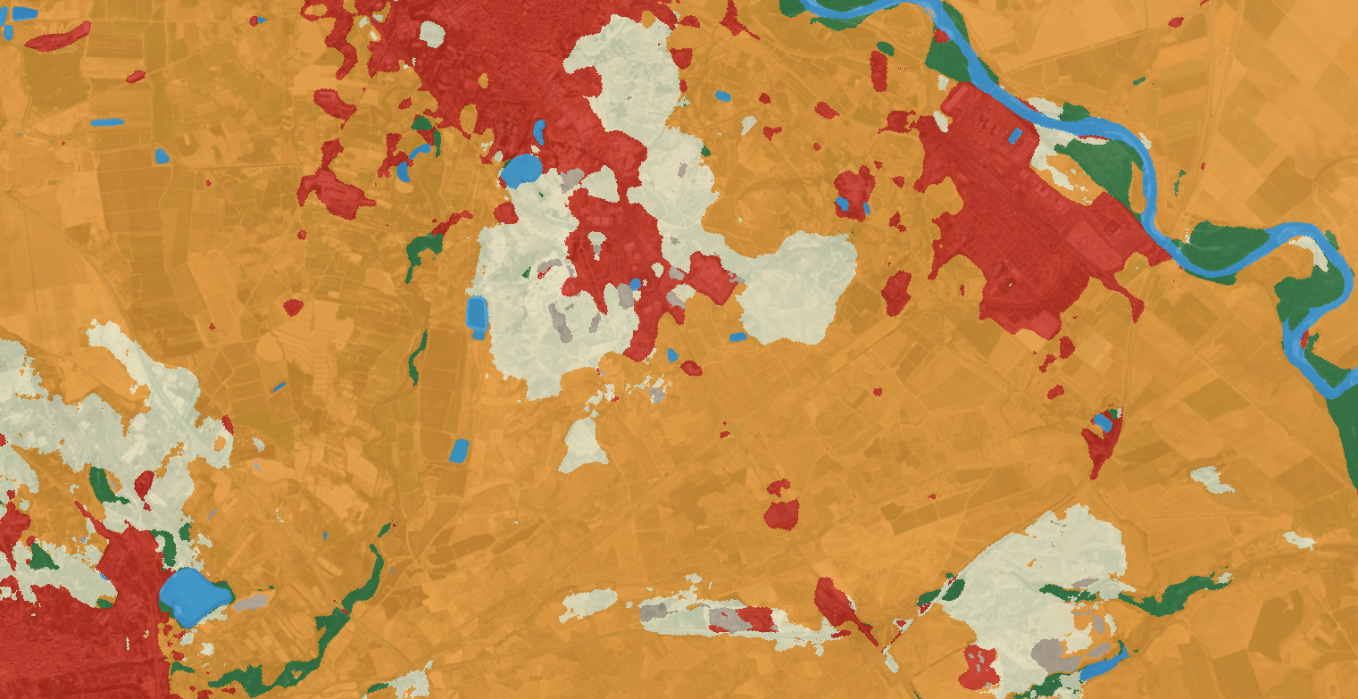
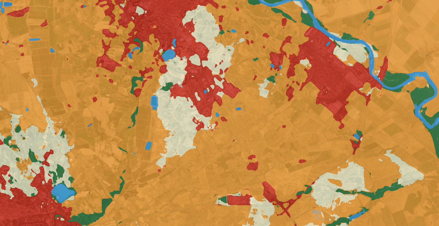
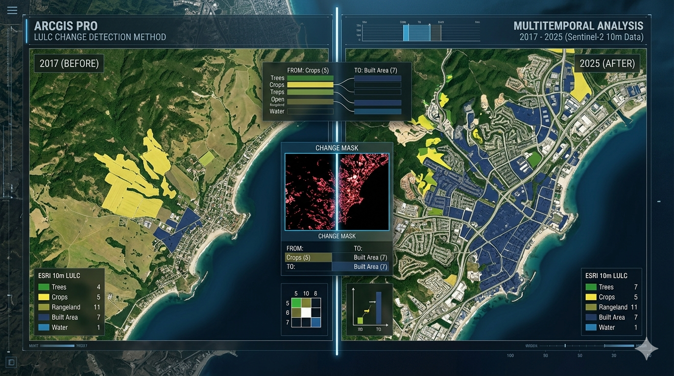
The quantification of land-use dynamics necessitates a spatiotemporal framework that ensures categorical stability over long-term observation windows. The ESRI 10-Meter Global Land Cover time series, accessible through the ArcGIS Living Atlas, provides a harmonized baseline for this purpose, derived from the dense temporal stack of the ESA Sentinel-2 mission.

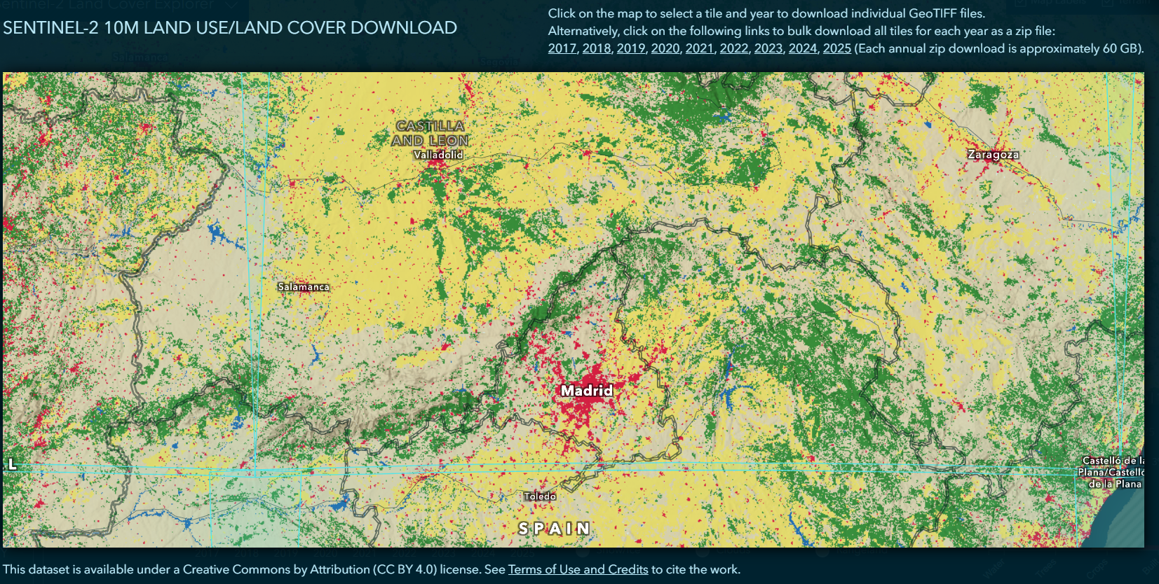
Since 2017, this dataset has utilized a consistent Deep Learning (U-Net) classification architecture, which is critical for mitigating the thematic noise often introduced by changing sensors or shifting methodologies. By maintaining a uniform 10-meter resolution and a standardized 9-class nomenclature, the series allows for a direct pixel-to-pixel comparison across years, enabling the identification of subtle urban expansion and environmental degradation without the requirement for secondary normalization or complex post-processing.

This repository is exposed via ArcGIS Pro as a series of multidimensional Image Services, a format that prioritizes computational efficiency through server-side processing. Rather than downloading massive raster tiles, the service allows for the direct execution of Pixel-Level Change Detection algorithms against the cloud-hosted imagery.

This “Open Data” approach facilitates a seamless transition from raw spectral data to actionable socio-spatial indicators. For researchers focusing on long-term urban trajectories, the continuity of this data from 2017 to the present ensures that the detected transitions reflect genuine terrestrial shifts rather than artifacts of the classification process. In an ArcGIS Pro environment, this translates to the ability to run Change Detection Raster Functions on-the-fly, producing transition matrices that quantify the conversion of permeable surfaces into built environments with high geographical precision and statistical rigor.

Analytical Implementation: Categorical Transition Matrices

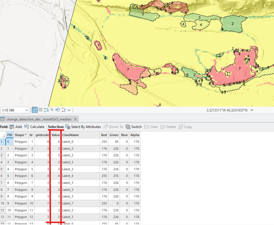
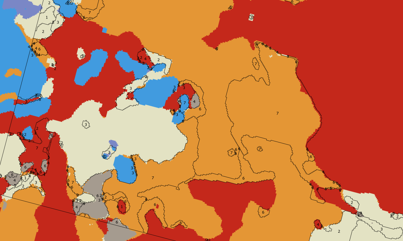
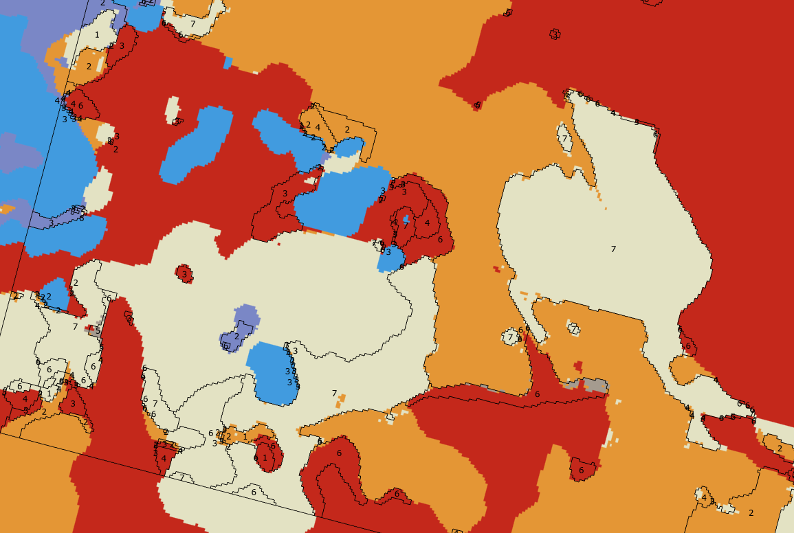
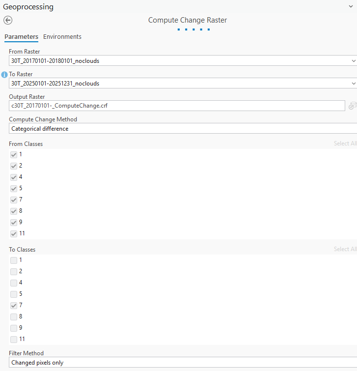
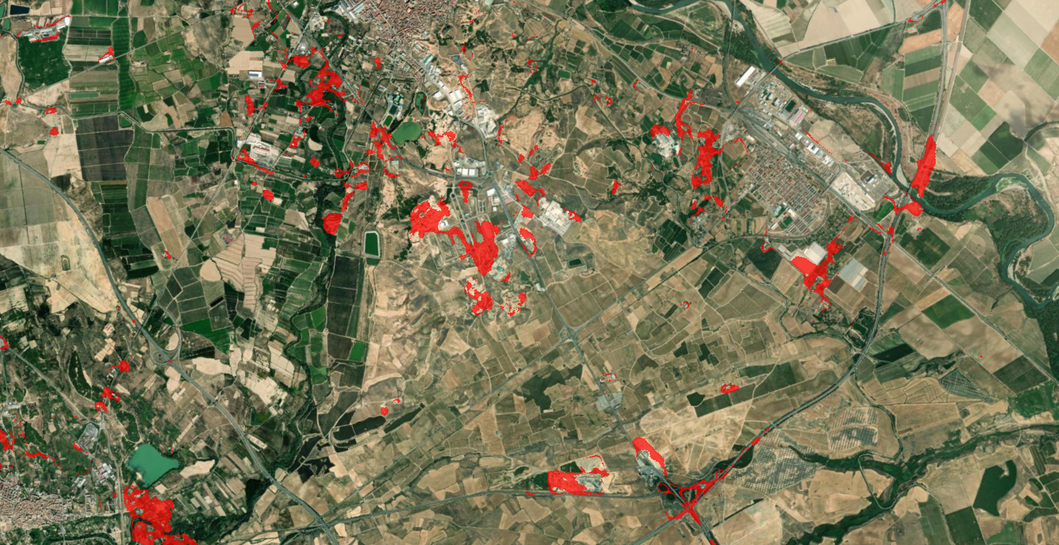
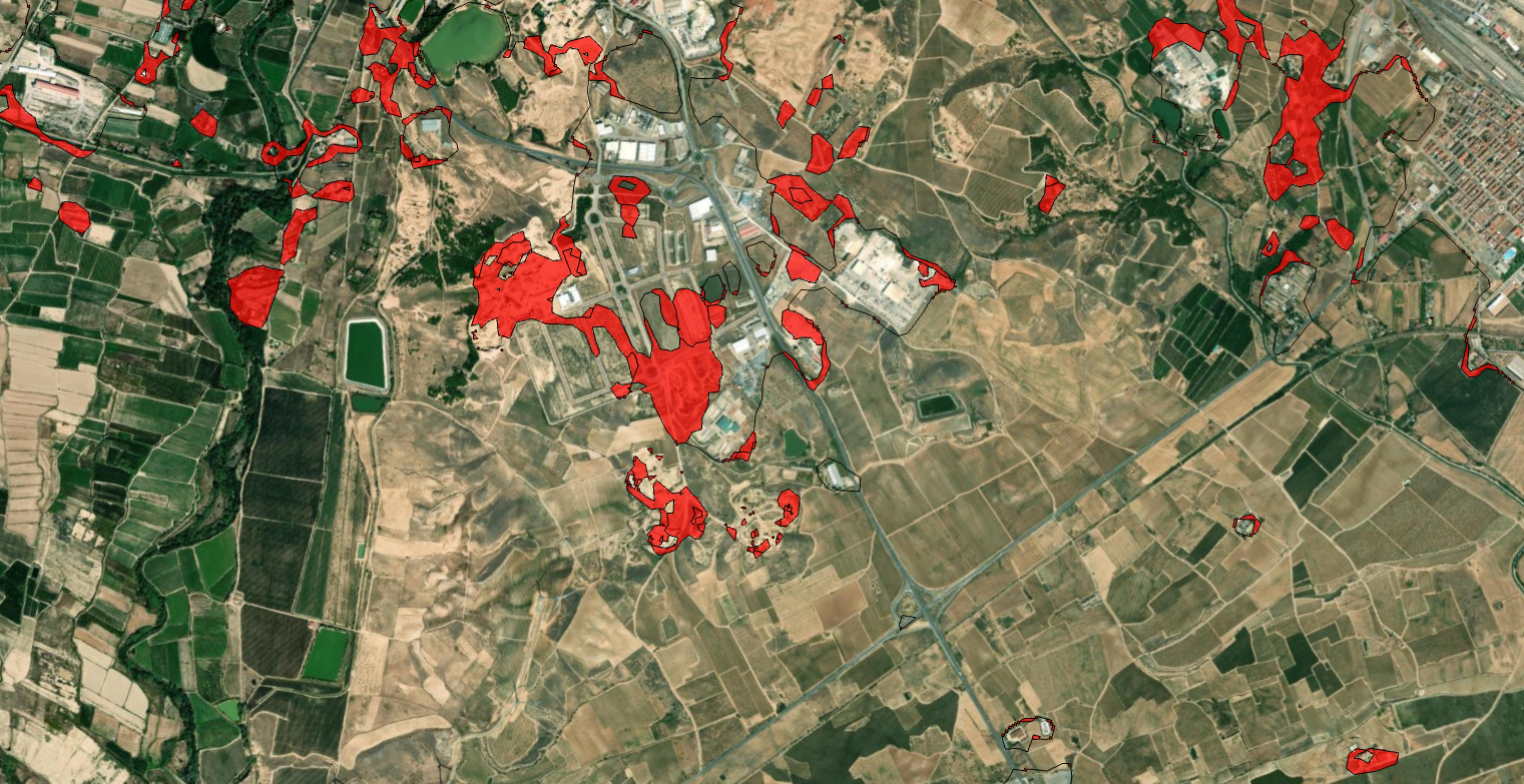
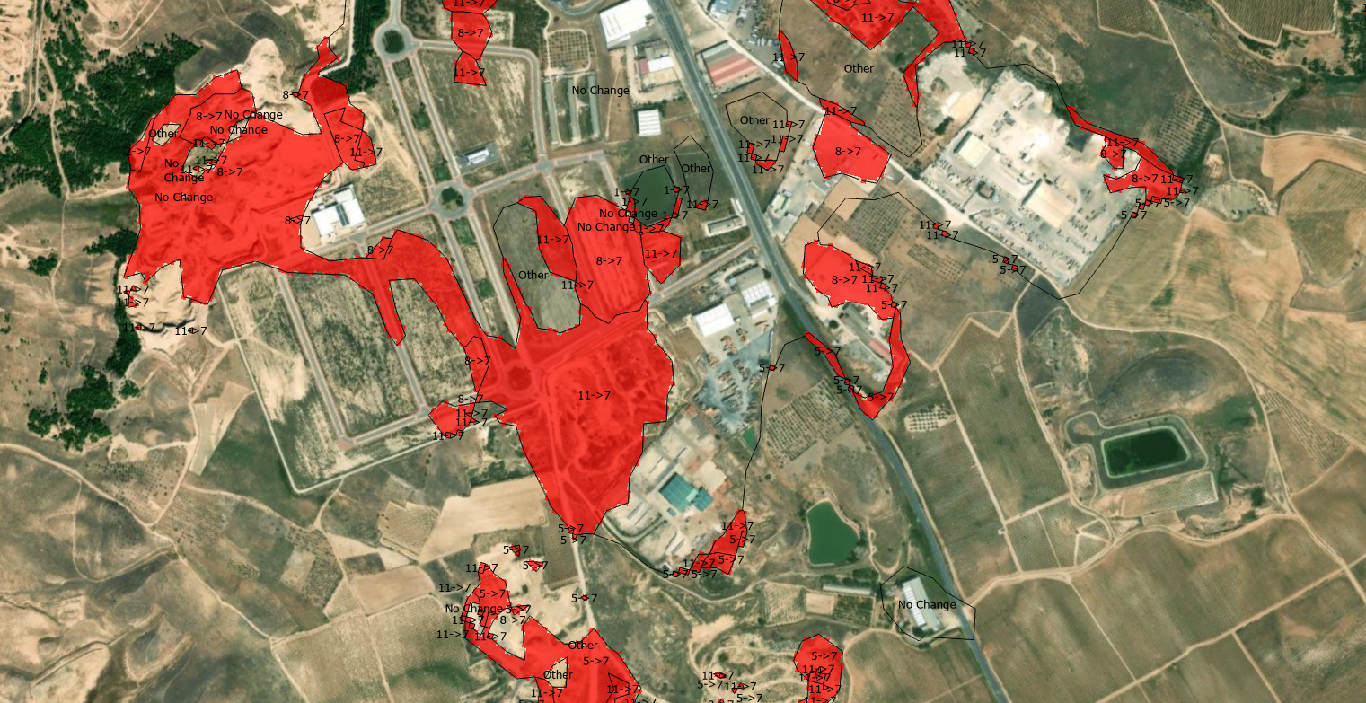
The core of the change detection workflow in ArcGIS Pro involves the application of the Compute Change Raster Function directly against the multidimensional Image Service slices. Unlike simple pixel subtraction used in spectral indices, categorical change detection requires the generation of a transition matrix to identify specific class-to-class trajectories. By defining the 2017 slice as the initial state and the current year as the final state, the software computes a thematic output where each pixel value represents a unique transition (e.g., Value 5 to Value 7, indicating the conversion of Crops to Built Area).

This process is optimized through the use of Raster Function Templates (RFTs), which allow for server-side processing of the Sentinel-2 derived layers. This avoids the latency of local data managed in geodatabases while maintaining the 10-meter spatial fidelity. For urban vulnerability research, this allows for the isolation of specific “vulnerability triggers”—such as the rapid expansion of impervious surfaces (Built Area) in areas previously classified as Flooded Vegetation (Class 4) or Water (Class 1). The resulting change raster is not merely a visual aid but a spatially explicit database capable of producing area-weighted statistics and frequency distributions that characterize the rate of urban transformation over the last decade.

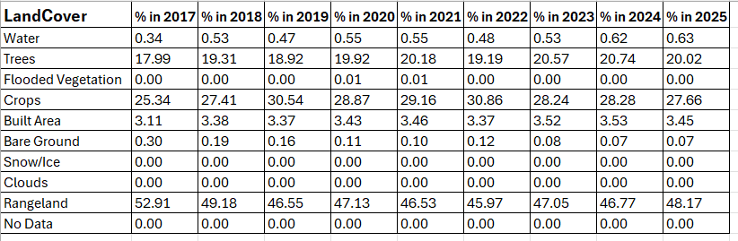
The integration of the ESRI 10-Meter Annual Land Cover series within ArcGIS Pro establishes a high-fidelity analytical pipeline for quantifying terrestrial transitions. By utilizing that consistent Deep Learning (U-Net) classification architecture across the Sentinel-2 archive from 2017 to the present, the dataset eliminates the methodological variances that typically compromise multi-temporal change detection. This longitudinal consistency is vital for isolating genuine socio-spatial shifts—such as the conversion of Rangeland (Class 11) or Crops (Class 5) into Built Area (Class 7)—from sensor-induced artifacts or classification drift.

Accessible as Open Data through the ArcGIS Living Atlas, these layers are delivered as multidimensional Image Services. This cloud-native architecture facilitates direct pixel-level interrogation without the prerequisite for local data ingestion or atmospheric correction. In a technical workflow, these services support the execution of Change Detection Raster Functions, enabling the generation of categorical transition matrices that intersect the 10-meter spatial resolution with the temporal depth of the Sentinel-2 mission. The result is a robust, replicable framework for monitoring urban sprawl, environmental vulnerability, and land-use governance with unprecedented statistical rigor.

Here is the full step-by-step procedure:

---

Step 1 — Load the rasters

1. Open ArcGIS Pro and create a new project or open an existing one
2. In the Catalog panel, navigate to your files
3. Drag and drop both files into the map:
   • 30T_20170101-20180101_noclouds
   • 30T_20250101-20251231_noclouds

---

Step 2 — Project to a metric CRS

1. Go to Analysis → Tools → search for Project Raster
2. Run it twice (once per raster):
   • Input Raster: 30T_20170101-20180101_noclouds
   • Output Raster: 30T_2017_projected.tif
   • Output Coordinate System: select your UTM zone (e.g. WGS 1984 UTM Zone 30N)
   • Resampling: Nearest (mandatory for classified rasters — never use Bilinear)
3. Repeat for 30T_20250101-20251231_noclouds → output 30T_2025_projected.tif

---

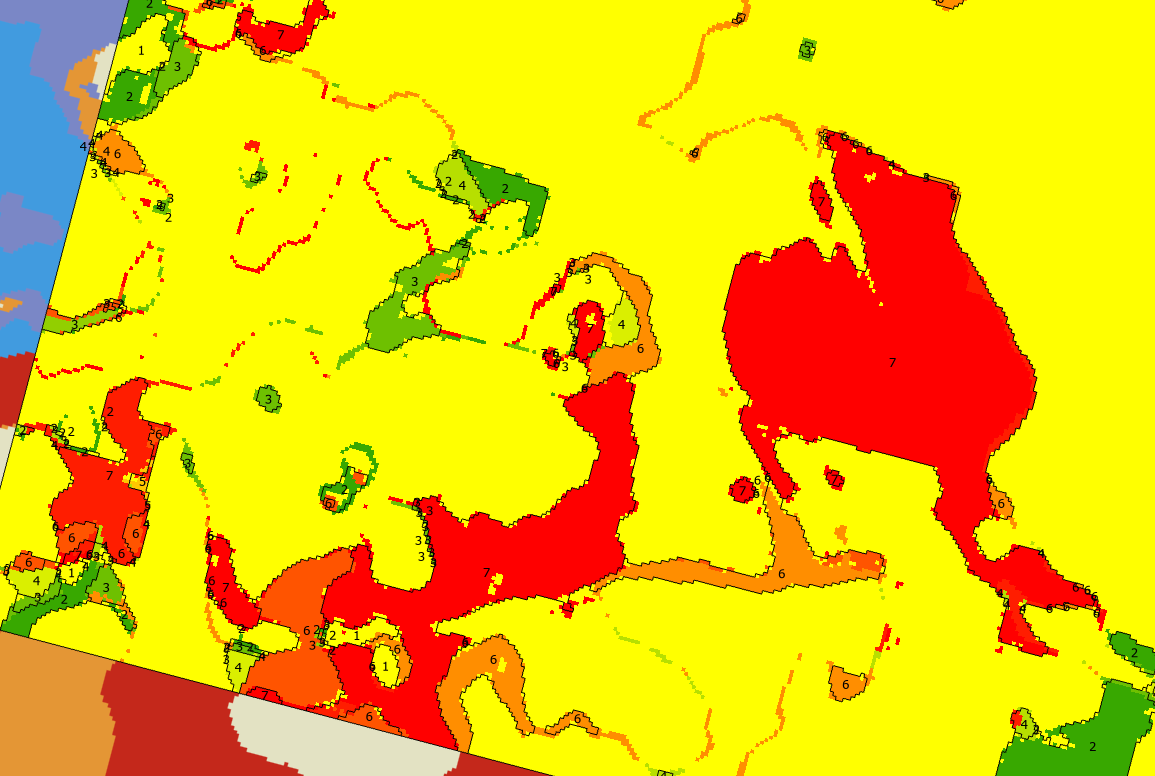
Step 3 — Run Compute Change Raster

1. Go to Analysis → Tools → search for Compute Change Raster
2. Fill in the parameters:

Parameter	Value
Input From Raster	30T_2017_projected.tif
Input To Raster	30T_2025_projected.tif
Compute Change Method	Categorical Difference
Filter Method	Changed pixels only
From Classes	(leave empty)
To Classes	7
Output Raster	change_urban_2017_2025.tif

3. Click Run

---

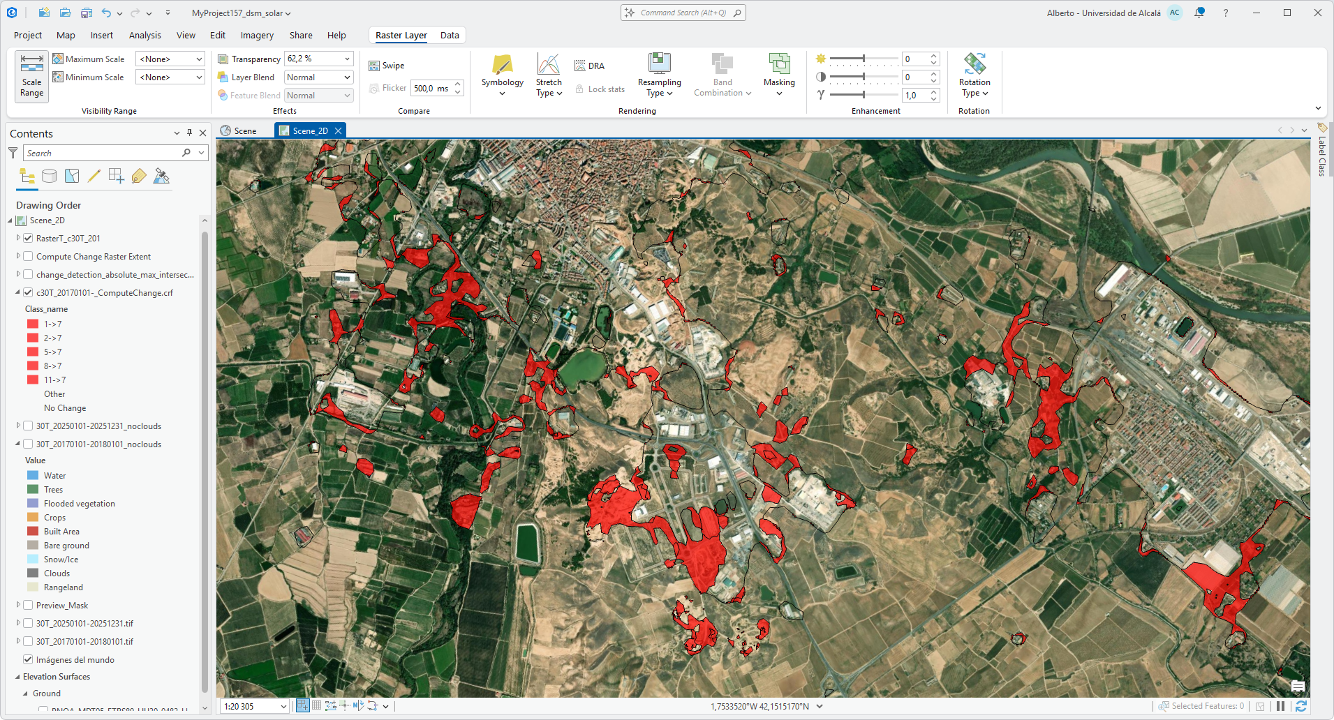
Step 4 — Symbolize the change layer

1. In the Contents panel, right-click change_urban_2017_2025.tif → Symbology
2. Set Primary symbology to Unique Values
3. Select all values in the color table → Ctrl+A
4. Right-click → Properties for all selected
5. Set color to #E82020 (or your preferred red)
6. Set outline to No Color
7. Close Symbology

---

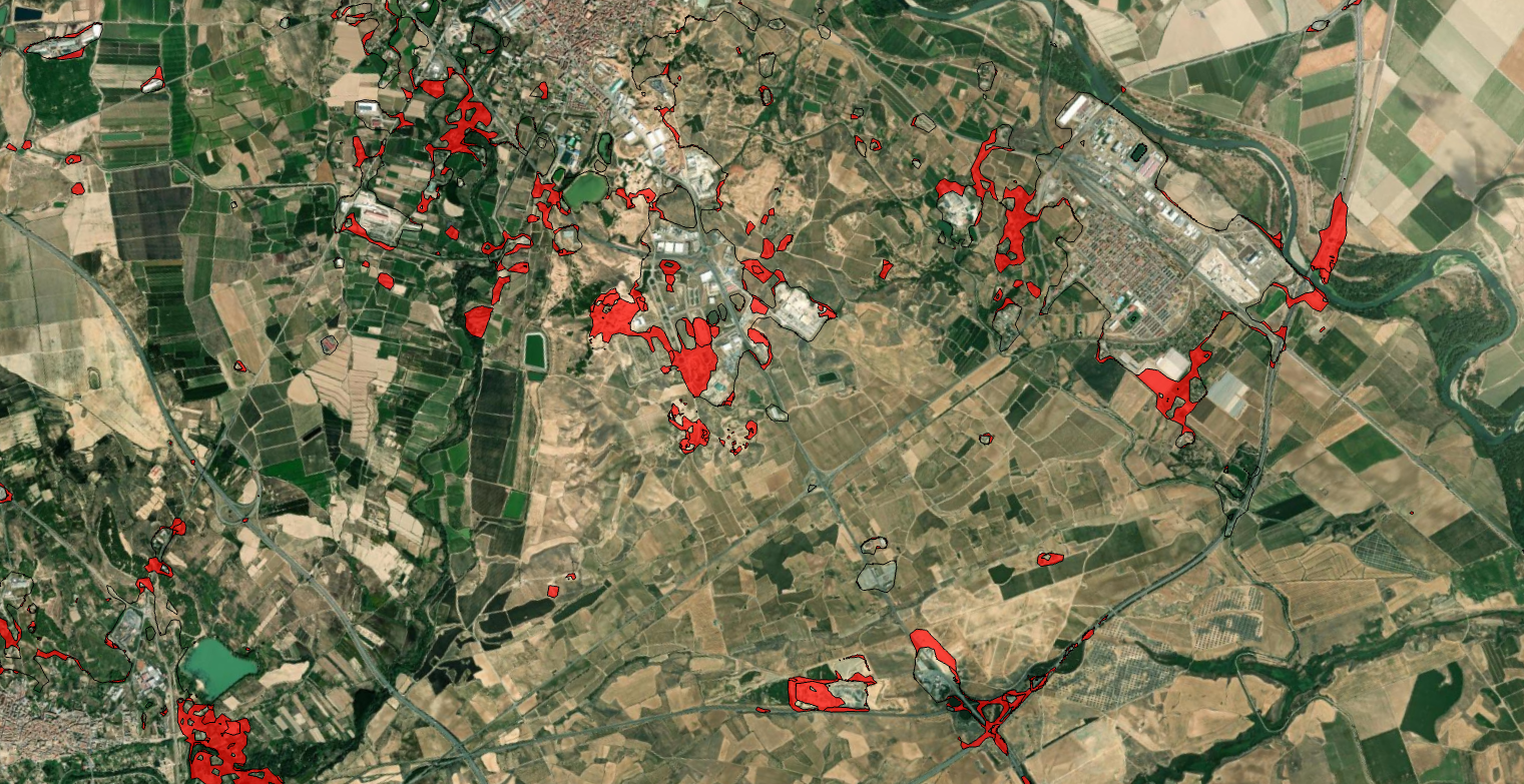
Step 5 — Add hillshade background

1. In the Contents panel, right-click the map → Add Data
2. Add a basemap: Map → Basemap → Light Gray Canvas (or any hillshade basemap)
3. In the Contents panel, drag change_urban_2017_2025.tif above the basemap
4. Right-click the change layer → Properties → Appearance
5. Set Transparency to 20%

Geographic Information Systems have transformed the way we understand territorial change, turning complex spatial phenomena into clear, measurable evidence. Tools like ArcGIS Pro consolidate in a single environment what once required multiple specialized software packages, reducing analysis time from days to minutes. The change detection workflow presented here — from raw classified rasters to a quantified urban growth map — was completed in under an hour, with no programming required.

This accessibility is key: it allows technicians, planners, and decision-makers to work with the same data and the same conclusions. Urban land monitoring is not a technical exercise in isolation; it feeds directly into land use planning, infrastructure investment, environmental impact assessment, and climate adaptation strategies. Knowing exactly where and how fast built-up area is expanding between two dates is information that governments, developers, and conservation agencies all need. The combination of freely available global products like the Esri Land Cover dataset with the analytical power of ArcGIS Pro and the Sentinel-2 satellite constellation has made this type of analysis accessible at any scale, from a municipality to an entire country. Change detection is not just a methodology — it is a way of making time visible on a map.

Interested in these change detection analysis? Let me know!

Alberto
GeoAI Analyst

https://www.arcgis.com/home/item.html?id=cfcb7609de5f478eb7666240902d4d3d

https://livingatlas.arcgis.com/landcoverexplorer/#mapCenter=147.74397%2C-37.18990%2C11.00&mode=step&timeExtent=2017%2C2025&year=2025