Why I Developed This Tool
Modern geospatial workflows increasingly depend on fast, reliable access to city-scale vector data — building footprints, road networks, land use polygons, points of interest, address databases. Whether you are designing a 5G radio network, modelling urban heat islands, planning last-mile logistics, or simulating emergency response coverage, you almost always start from the same question: “How do I get clean, structured geodata for this city, right now, without spending two days on it?”
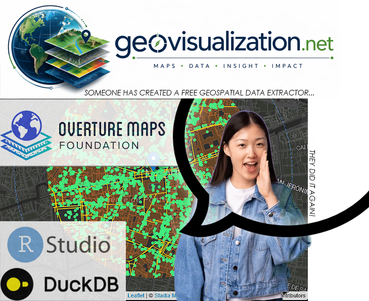
The Overture Maps Extractor is my answer to that question. It is a Shiny application written in R that lets any GIS professional extract multiple thematic layers from the Overture Maps Foundation dataset — for any city in the world — in a matter of minutes, with zero command-line interaction and zero manual data wrangling.
What Is Overture Maps?
The Overture Maps Foundation is an open data initiative backed by Amazon, Meta, Microsoft and TomTom. It publishes a continuously updated, globally consistent vector dataset covering:
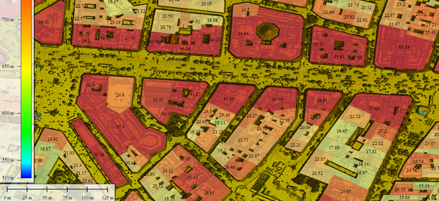
- Buildings — footprints with height and floor count attributes where available
- Transportation — roads, railways, and hydrography segments
- Places (POIs) — points of interest with categories and confidence scores
- Addresses — street-level address points with number, postcode and city
- Land Use / LULC — polygonal land cover classification
- Administrative divisions — municipal and regional boundaries
- Base land features — parks, forests, water bodies as polygons
- Infrastructure — energy towers, antennas, utilities
The data is published as GeoParquet files on Amazon S3, updated with every release cycle. The latest release as of this writing is 2026-04-15.0.
The Technical Stack: R + DuckDB + Overture Maps
The core of the extractor is a single R Shiny application. No Python, no Docker, no cloud infrastructure required — just a running R session.
DuckDB as the Query Engine
The key enabler is DuckDB, an in-process analytical database that can query remote Parquet files over HTTP range requests without downloading the entire dataset. A city-scale extraction that would otherwise require gigabytes of data transfer is reduced to fetching only the relevant row groups.
r
dbExecute(con, "INSTALL httpfs; LOAD httpfs;")dbExecute(con, "INSTALL spatial; LOAD spatial;")dbExecute(con, "SET s3_region='us-west-2';")
The spatial filter is pushed directly into the Parquet scan via bounding box predicates on the bbox struct columns — a pattern that Overture’s file layout is specifically optimised for. Overture’s latest schema exposes native GEOMETRY('OGC:CRS84') types, which DuckDB Spatial handles natively via ST_AsText() for clean WKT export to R sf objects.
In this particular case of a spanish scenario over Madrid, we have DTM/DSM Open Data from CNIG, then we can easily get AGL heights from a raster difference (DSM-DTM).
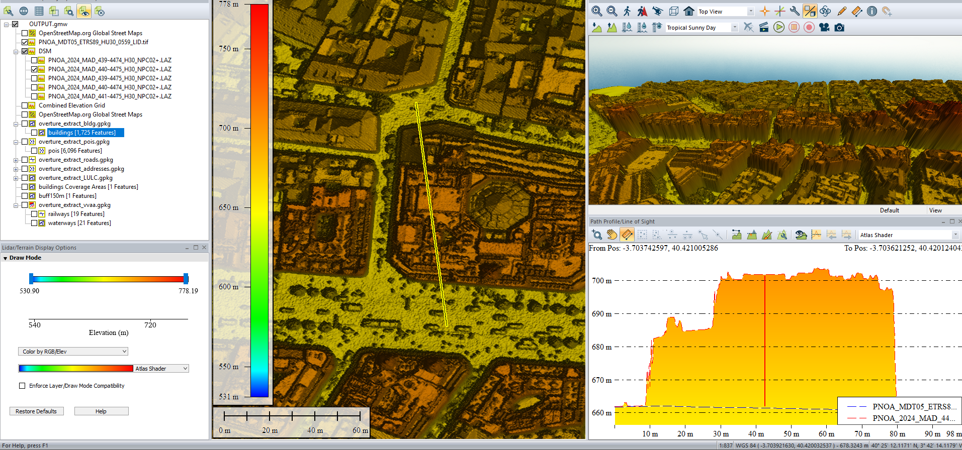
Yes, you are right, I did it using global Mapper.
Workflow in Three Steps
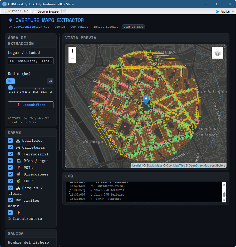
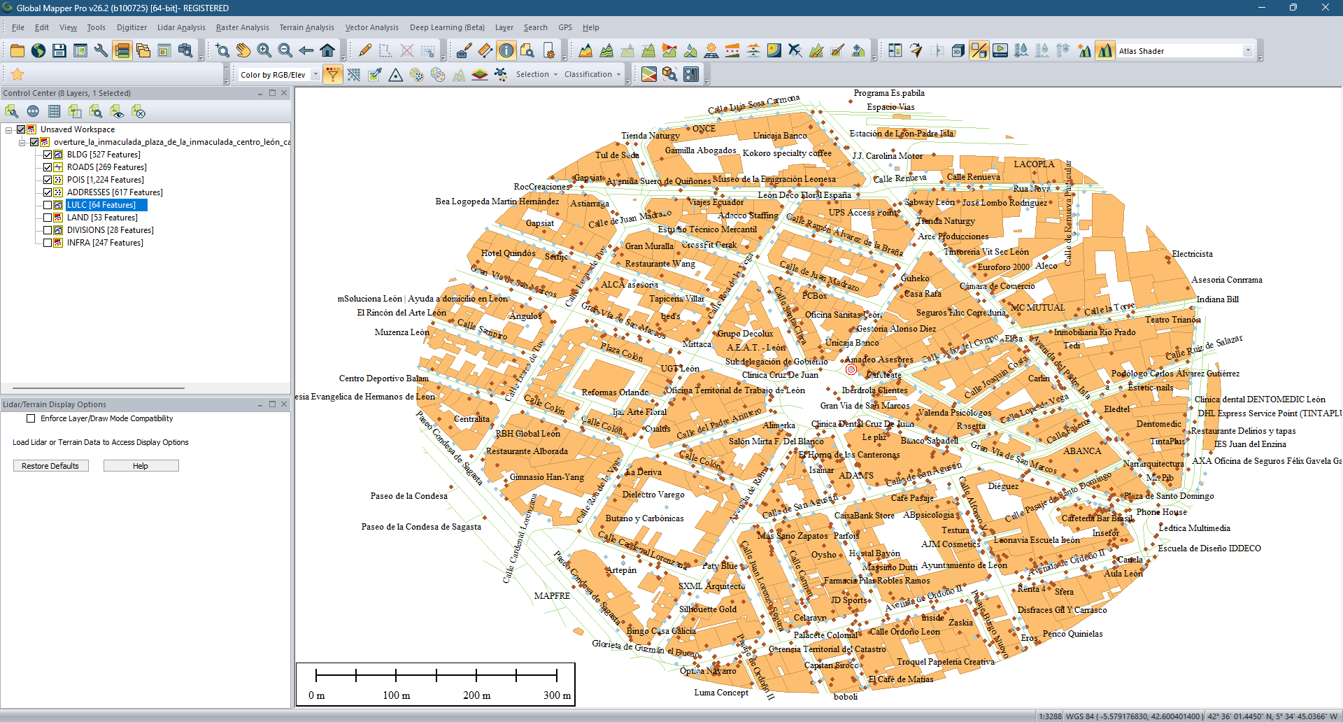
1. Locate — type a city name (or drag the interactive marker anywhere on the map) and set a radius in kilometres. The application geocodes via OpenStreetMap Nominatim and computes a circular extraction area using a proper metric buffer in EPSG:3857, avoiding the distortion of a simple bounding box.
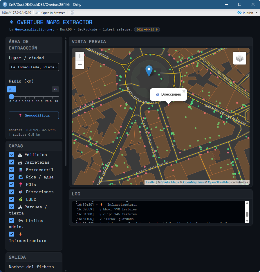
2. Select layers — toggle any combination of the ten available thematic layers with checkboxes.
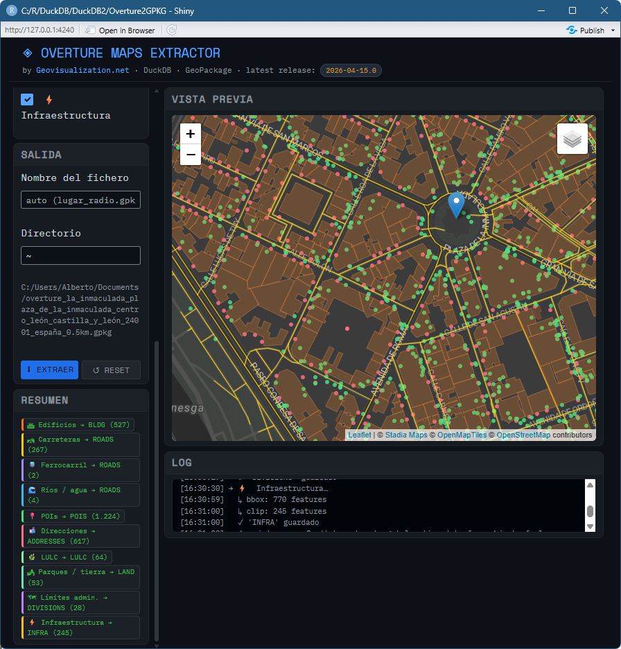
3. Extract — a single button press launches the DuckDB queries, clips the results to the circular area, and writes everything to a single OGC GeoPackage (.gpkg) with standardised layer names: BLDG, ROADS, POIS, ADDRESSES, LULC, LAND, DIVISIONS, INFRA.
The output is immediately ready for QGIS, ArcGIS Pro, PostGIS, or any OGC-compliant GIS tool.
Applications Across Domains
Smart Cities & Urban Analytics Building footprints combined with LULC and POI density form the backbone of urban morphology analysis — walkability indices, urban heat island modelling, green space accessibility, population exposure estimation.
Telecommunications & Radio Planning For 5G and LTE network planning, building height data directly feeds propagation models (ITU-R P.1411, COST-Hata). Address layers enable subscriber geocoding and coverage gap analysis. Road network topology supports site accessibility routing. The circular extraction pattern maps directly to cell sector coverage radii.
Emergency Management & Resilience First-responder route optimisation, shelter location analysis, flood exposure by building footprint — all start from the same data layers this tool produces in minutes.
Real Estate & Infrastructure Investment Rapid assessment of urban fabric density, street connectivity, and amenity proximity for any candidate city worldwide, with a consistent schema regardless of country.
OGC GeoPackage: The Right Output Format
The output format is deliberately OGC GeoPackage — a single SQLite-based file that is fully OGC-compliant, contains all layers, preserves CRS metadata (EPSG:4326), and requires no proprietary software to open. It is the format of choice for field deployment, data exchange, and reproducible workflows.
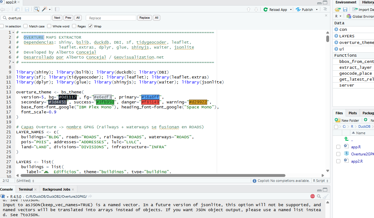
Do you want to code it yourself?. I herewith give you my code:
r
# =============================================================================# OVERTURE MAPS EXTRACTOR# Dependencies: shiny, bslib, duckdb, DBI, sf, tidygeocoder, leaflet,# leaflet.extras, dplyr, glue, shinyjs, waiter, jsonlite# Developed by Alberto Concejal / Geovisualization.net # =============================================================================library(shiny); library(bslib); library(duckdb); library(DBI)library(sf); library(tidygeocoder); library(leaflet); library(leaflet.extras)library(dplyr); library(glue); library(shinyjs); library(waiter); library(jsonlite)overture_theme <- bs_theme( version=5, bg="#0d1117", fg="#e6edf3", primary="#58a6ff", secondary="#3d4451", success="#3fb950", danger="#f85149", warning="#d29922", base_font=font_google("IBM Plex Mono"), heading_font=font_google("Space Mono"), font_scale=0.9)# Capas Overture -> nombre GPKG (railways + waterways se fusionan en ROADS)LAYER_NAMES <- c( buildings="BLDG", roads="ROADS", railways="ROADS", waterways="ROADS", pois="POIS", addresses="ADDRESSES", lulc="LULC", land="LAND", divisions="DIVISIONS", infrastructure="INFRA")LAYERS <- list( buildings = list( label="🏛 Edificios", theme="buildings", type="building", fields='id, names."primary" AS name, height, num_floors, class, ST_AsText(geometry) AS geom_wkt' ), roads = list( label="🛣 Carreteras", theme="transportation", type="segment", fields='id, names."primary" AS name, class, subtype, ST_AsText(geometry) AS geom_wkt', filter="AND subtype = 'road'" ), railways = list( label="🚆 Ferrocarril", theme="transportation", type="segment", fields='id, names."primary" AS name, class, subtype, ST_AsText(geometry) AS geom_wkt', filter="AND subtype = 'rail'" ), waterways = list( label="🌊 Ríos / agua", theme="base", type="water", fields='id, names."primary" AS name, subtype, class, ST_AsText(geometry) AS geom_wkt' ), pois = list( label="📍 POIs", theme="places", type="place", fields='id, names."primary" AS name, basic_category AS category, confidence, ST_AsText(geometry) AS geom_wkt' ), addresses = list( label="📬 Direcciones", theme="addresses", type="address", fields='id, street, number, postcode, postal_city, country, ST_AsText(geometry) AS geom_wkt' ), lulc = list( label="🌿 LULC", theme="base", type="land_use", fields='id, names."primary" AS name, subtype, class, ST_AsText(geometry) AS geom_wkt' ), land = list( label="🏞 Parques / tierra", theme="base", type="land", fields='id, names."primary" AS name, subtype, class, ST_AsText(geometry) AS geom_wkt' ), divisions = list( label="🗺 Límites admin.", theme="divisions", type="division_area", fields='id, names."primary" AS name, subtype, admin_level, ST_AsText(geometry) AS geom_wkt' ), infrastructure = list( label="⚡ Infraestructura", theme="base", type="infrastructure", fields='id, names."primary" AS name, subtype, class, ST_AsText(geometry) AS geom_wkt' ))# Colores por capa (también usados en el control de capas del mapa)LAYER_COLORS <- c( buildings="#f97316", roads="#facc15", railways="#a78bfa", waterways="#38bdf8", pois="#4ade80", addresses="#fb7185", lulc="#86efac", land="#6ee7b7", divisions="#c084fc", infrastructure="#fbbf24")# ---- Helpers -----------------------------------------------------------------get_latest_release <- function() { tryCatch(jsonlite::fromJSON("https://stac.overturemaps.org/catalog.json")$latest, error=function(e) "2026-04-15.0")}geocode_place <- function(place_name) { res <- tidygeocoder::geo(address=place_name, method="osm", full_results=FALSE, quiet=TRUE) if (nrow(res)==0 || is.na(res$long)) return(NULL) c(lon=res$long, lat=res$lat)}bbox_from_center <- function(lon, lat, buffer_km) { dlat <- buffer_km / 111.32 dlon <- buffer_km / (111.32 * cos(lat * pi / 180)) list(xmin=lon-dlon, ymin=lat-dlat, xmax=lon+dlon, ymax=lat+dlat)}circle_from_center <- function(lon, lat, buffer_km) { st_sfc(st_point(c(lon, lat)), crs=4326) |> st_transform(3857) |> st_buffer(buffer_km * 1000, nQuadSegs=32) |> st_transform(4326)}extract_layer <- function(con, layer_id, bbox, release) { cfg <- LAYERS[[layer_id]] s3 <- glue("s3://overturemaps-us-west-2/release/{release}/theme={cfg$theme}/type={cfg$type}/*") extra <- if (!is.null(cfg$filter)) cfg$filter else "" sql <- glue(" SELECT {cfg$fields} FROM read_parquet('{s3}', filename=true, hive_partitioning=1) WHERE bbox.xmin <= {bbox$xmax} AND bbox.xmax >= {bbox$xmin} AND bbox.ymin <= {bbox$ymax} AND bbox.ymax >= {bbox$ymin} {extra} ") tryCatch({ df <- dbGetQuery(con, sql) if (nrow(df)==0) return(NULL) st_as_sf(df, wkt="geom_wkt", crs=4326) }, error=function(e) { message("[",layer_id,"] ",conditionMessage(e)); NULL })}clip_to_circle <- function(sf_obj, circle_sf) { tryCatch({ cl <- st_intersection(st_make_valid(sf_obj), circle_sf) if (nrow(cl)==0) NULL else cl }, error=function(e) { message("clip: ",conditionMessage(e)); sf_obj })}write_gpkg_layer <- function(sf_obj, out_path, layer_name) { sf_obj <- sf_obj |> select(where(~!is.list(.x))) sf::st_write(sf_obj, out_path, layer=layer_name, driver="GPKG", delete_layer=TRUE, quiet=TRUE)}# Nombre de fichero por defecto basado en lugar y radiodefault_filename <- function(place, km) { slug <- place |> tolower() |> gsub("[^a-z0-9áéíóúñ ]", "", x=_) |> trimws() |> gsub("\\s+", "_", x=_) paste0("~/overture_", slug, "_", km, "km.gpkg")}# ---- UI ----------------------------------------------------------------------ui <- fluidPage( theme=overture_theme, useShinyjs(), useWaiter(), tags$head(tags$style(HTML(" html, body { background:#0d1117; height:100%; overflow:hidden; } .container-fluid { height:100%; } .app-header { border-bottom:1px solid #21262d; padding:0.5rem 1.2rem 0.4rem; margin-bottom:0.5rem } .app-title { font-family:'Space Mono',monospace; font-size:1.2rem; color:#58a6ff; letter-spacing:-0.5px } .app-subtitle { color:#8b949e; font-size:0.7rem; margin-top:1px } /* columna izquierda: scroll interno si no cabe */ .left-col { height: calc(100vh - 70px); overflow-y: auto; overflow-x: hidden; padding-right: 6px; scrollbar-width: thin; scrollbar-color: #30363d #0d1117; } .left-col::-webkit-scrollbar { width:4px } .left-col::-webkit-scrollbar-track { background:#0d1117 } .left-col::-webkit-scrollbar-thumb { background:#30363d; border-radius:2px } .card { background:#161b22!important; border:1px solid #21262d!important; margin-bottom:0.4rem!important } .card-header { background:#1c2128!important; border-bottom:1px solid #21262d!important; font-family:'Space Mono',monospace; font-size:0.72rem; color:#8b949e; text-transform:uppercase; letter-spacing:1px; padding:0.28rem 0.65rem!important } .card-body { padding:0.4rem 0.65rem!important } .layer-check .form-check { margin-bottom:0.12rem } .layer-check .form-check-label { font-size:0.78rem } .form-label { font-size:0.78rem; margin-bottom:0.12rem } .form-control { font-size:0.78rem; padding:0.18rem 0.4rem } .form-range { padding:0 } .btn-sm { font-size:0.75rem; padding:0.15rem 0.4rem } #geocode_btn { font-size:0.75rem; padding:0.18rem 0.4rem } #extract_btn { font-family:'Space Mono',monospace; background:#1f6feb; border:none; font-size:0.78rem; padding:0.25rem 0.5rem; white-space:nowrap } #extract_btn:hover { background:#388bfd } #reset_btn { font-family:'Space Mono',monospace; background:#21262d; border:1px solid #30363d; font-size:0.75rem; padding:0.22rem 0.5rem; color:#8b949e; white-space:nowrap } #reset_btn:hover { background:#30363d; color:#e6edf3 } .btn-row { display:flex; gap:5px; margin-top:5px } .btn-row .btn { flex:1; min-width:0 } .log-box { background:#010409; border:1px solid #21262d; border-radius:6px; padding:0.4rem 0.65rem; font-size:0.67rem; color:#8b949e; font-family:'IBM Plex Mono',monospace; height:78px; overflow-y:auto; white-space:pre-wrap } .stat-badge { display:inline-block; background:#1c2128; border:1px solid #30363d; border-radius:4px; padding:1px 5px; font-size:0.63rem; color:#3fb950; margin:1px; font-family:'IBM Plex Mono',monospace } .release-badge { display:inline-block; background:#1f2937; border:1px solid #374151; border-radius:12px; padding:1px 7px; font-size:0.63rem; color:#d29922; font-family:'IBM Plex Mono',monospace } .leaflet-container { border-radius:6px } .irs--shiny .irs-bar { height:3px } .irs--shiny .irs-line { height:3px } .irs--shiny .irs-handle { top:22px } .irs-min, .irs-max, .irs-single { font-size:0.67rem } "))), div(class="app-header", div(class="app-title", "◈ OVERTURE MAPS EXTRACTOR"), div(class="app-subtitle", "by ", tags$a("Geovisualization.net", href="https://geovisualization.net", target="_blank", style="color:#58a6ff;text-decoration:none;"), " · DuckDB · GeoPackage · latest release: ", uiOutput("release_badge", inline=TRUE) ) ), fluidRow(style="margin:0", # ---- Columna izquierda --------------------------------------------------- column(3, class="left-col", style="padding-left:6px", card(card_header("Área de extracción"), card_body( textInput("place_name", "Lugar / ciudad", value="Madrid, España"), sliderInput("buffer_km", "Radio (km)", min=0.5, max=25, value=3, step=0.5), actionButton("geocode_btn", "📍 Geocodificar", class="btn btn-outline-primary btn-sm w-100 mb-1"), div(style="font-size:0.7rem;color:#8b949e;line-height:1.4;margin-top:2px", textOutput("bbox_info")) )), card(card_header("Capas"), card_body(padding="0.35rem", div(class="layer-check", checkboxGroupInput("layers_sel", label=NULL, choices=setNames(names(LAYERS), sapply(LAYERS,`[[`,"label")), selected=c("buildings","roads","pois"))) )), card(card_header("Salida"), card_body( textInput("filename_base", "Nombre del fichero", value="", placeholder="auto (lugar_radio.gpkg)"), textInput("out_dir", "Directorio", value="~"), div(style="font-size:0.68rem;color:#8b949e;margin-bottom:4px", textOutput("out_path_preview")), div(class="btn-row", actionButton("extract_btn", "⬇ EXTRAER", class="btn btn-primary"), actionButton("reset_btn", "↺ RESET", class="btn") ) )), card(card_header("Resumen"), card_body(uiOutput("stats_ui"))) ), # ---- Columna derecha ----------------------------------------------------- column(9, style="padding-left:6px", card(card_header("Vista previa"), card_body(padding=0, leafletOutput("preview_map", height="470px"))), card(class="mt-2", card_header("Log"), card_body(padding="0.35rem", div(class="log-box", id="log_box", textOutput("log_text")))) ) ))# ---- Server ------------------------------------------------------------------server <- function(input, output, session) { rv <- reactiveValues( lon=(-3.7038), lat=40.4168, bbox=NULL, circle=NULL, logs=character(0), results=list(), release="…" ) output$release_badge <- renderUI(tags$span(class="release-badge", rv$release)) observe({ rv$release <- isolate(get_latest_release()) }) # Logger add_log <- function(msg) { rv$logs <- c(rv$logs, paste0("[",format(Sys.time(),"%H:%M:%S"),"] ",msg)) } output$log_text <- renderText(paste(tail(rv$logs, 60), collapse="\n")) observe({ rv$logs shinyjs::runjs("var l=document.getElementById('log_box');if(l)l.scrollTop=l.scrollHeight;") }) # Ruta de salida calculada get_out_path <- reactive({ base <- trimws(input$filename_base) dir <- trimws(input$out_dir) if (dir=="") dir <- "~" if (base=="") { base <- default_filename(input$place_name, input$buffer_km) base <- basename(base) } if (!grepl("\\.gpkg$", base, ignore.case=TRUE)) base <- paste0(base, ".gpkg") path.expand(file.path(dir, base)) }) output$out_path_preview <- renderText({ get_out_path() }) # Mapa base con control de capas output$preview_map <- renderLeaflet({ leaflet(options=leafletOptions(preferCanvas=TRUE)) %>% # Basemap oscuro con etiquetas en inglés addProviderTiles("Stadia.AlidadeSmoothDark", options=tileOptions(opacity=0.95)) %>% setView(lng=rv$lon, lat=rv$lat, zoom=13) %>% # Marker arrastrable en posición inicial addMarkers( lng=rv$lon, lat=rv$lat, layerId="center_marker", options=markerOptions(draggable=TRUE), label="Drag to reposition" ) %>% addLayersControl( overlayGroups = names(LAYERS), options = layersControlOptions(collapsed=TRUE) ) }) # Cuando el marker se suelta en nueva posición observeEvent(input$preview_map_marker_dragend, { info <- input$preview_map_marker_dragend req(info$id == "center_marker") rv$lon <- info$lng rv$lat <- info$lat rv$bbox <- bbox_from_center(rv$lon, rv$lat, input$buffer_km) rv$circle <- circle_from_center(rv$lon, rv$lat, input$buffer_km) add_log(sprintf("📌 Marcador movido → %.5f, %.5f", rv$lon, rv$lat)) # Reverse geocode para actualizar el campo de texto tryCatch({ res <- tidygeocoder::reverse_geo( lat=rv$lat, long=rv$lon, method="osm", full_results=FALSE, quiet=TRUE ) if (nrow(res)>0 && !is.na(res$address)) { updateTextInput(session, "place_name", value=res$address) add_log(paste(" ↳ lugar:", res$address)) } }, error=function(e) NULL) updateTextInput(session, "filename_base", value="") update_map_circle() }) # Geocodificar observeEvent(input$geocode_btn, { req(nchar(trimws(input$place_name))>0) add_log(paste("Geocodificando:", input$place_name)) coords <- withProgress(message="Geocodificando…", value=0.5, geocode_place(input$place_name)) if (is.null(coords)) { add_log("⚠ Sin coordenadas. Prueba con nombre más específico") add_log(" ej: 'León, Castilla y León, España' o arrastra el marcador") showNotification("Geocodificación fallida — prueba a arrastrar el marcador", type="warning", duration=5) return() } rv$lon <- coords["lon"]; rv$lat <- coords["lat"] rv$bbox <- bbox_from_center(rv$lon, rv$lat, input$buffer_km) rv$circle <- circle_from_center(rv$lon, rv$lat, input$buffer_km) add_log(sprintf("✓ %.5f, %.5f | radio: %g km", rv$lon, rv$lat, input$buffer_km)) updateTextInput(session, "filename_base", value="") update_map_circle() }) observeEvent(input$buffer_km, { if (!is.null(rv$bbox)) { rv$bbox <- bbox_from_center(rv$lon, rv$lat, input$buffer_km) rv$circle <- circle_from_center(rv$lon, rv$lat, input$buffer_km) update_map_circle() } }) update_map_circle <- function() { b <- rv$bbox leafletProxy("preview_map") %>% clearShapes() %>% # Redibujar círculo addCircles(lng=rv$lon, lat=rv$lat, radius=input$buffer_km*1000, fillColor="transparent", color="#58a6ff", weight=1.5, dashArray="4") %>% # Mover marker arrastrable a nueva posición removeMarker("center_marker") %>% addMarkers(lng=rv$lon, lat=rv$lat, layerId="center_marker", options=markerOptions(draggable=TRUE), label="Drag to reposition") %>% flyToBounds(b$xmin, b$ymin, b$xmax, b$ymax) } output$bbox_info <- renderText({ if (is.null(rv$bbox)) return("No area set") sprintf("center: %.4f, %.4f | radius: %g km", rv$lon, rv$lat, input$buffer_km) }) # Reset observeEvent(input$reset_btn, { rv$lon <- -3.7038; rv$lat <- 40.4168 rv$bbox <- bbox_from_center(rv$lon, rv$lat, 3) rv$circle <- circle_from_center(rv$lon, rv$lat, 3) rv$results <- list() rv$logs <- character(0) updateTextInput(session, "place_name", value="Madrid, España") updateTextInput(session, "filename_base", value="") updateTextInput(session, "out_dir", value="~") updateSliderInput(session, "buffer_km", value=3) updateCheckboxGroupInput(session, "layers_sel", selected=c("buildings","roads","pois")) leafletProxy("preview_map") %>% clearShapes() %>% removeMarker("center_marker") %>% clearGroup(names(LAYERS)) %>% addMarkers(lng=-3.7038, lat=40.4168, layerId="center_marker", options=markerOptions(draggable=TRUE), label="Drag to reposition") %>% setView(lng=-3.7038, lat=40.4168, zoom=13) add_log("↺ Reset — ready for new extraction") }) # Extracción observeEvent(input$extract_btn, { req(!is.null(rv$bbox), !is.null(rv$circle), length(input$layers_sel)>0) layers <- input$layers_sel bbox <- rv$bbox circle <- rv$circle release <- rv$release out_path <- get_out_path() add_log("── Iniciando extracción ──────────────────────") add_log(paste("Release:", release)) add_log(paste("Capas:", paste(layers, collapse=", "))) add_log(paste("Salida:", out_path)) rv$results <- list() # ── DuckDB: conexión explícita con cierre garantizado ────────────────── # Usamos un bloque local + tryCatch para garantizar dbDisconnect # aunque falle cualquier query individual con <- NULL tryCatch({ con <- dbConnect(duckdb::duckdb(), dbdir=":memory:") dbExecute(con, "INSTALL httpfs; LOAD httpfs;") dbExecute(con, "INSTALL spatial; LOAD spatial;") dbExecute(con, "SET s3_region='us-west-2';") dbExecute(con, "SET memory_limit='3GB';") dbExecute(con, "SET threads=2;") # evitar saturar RAM con paralelismo dbExecute(con, "SET http_timeout=120000;") # 120 s timeout S3 add_log("✓ DuckDB listo") }, error=function(e) { add_log(paste("✗ DuckDB init error:", conditionMessage(e))) if (!is.null(con)) try(dbDisconnect(con, shutdown=TRUE), silent=TRUE) return() }) # Limpiar capas anteriores del mapa leafletProxy("preview_map") %>% clearGroup(names(LAYERS)) withProgress(message="Extracting from Overture…", value=0, { for (i in seq_along(layers)) { lid <- layers[i] add_log(paste0("→ ", LAYERS[[lid]]$label, "…")) incProgress(1/length(layers), detail=LAYERS[[lid]]$label) # ── 1. Query DuckDB (protegida individualmente) ────────────────── sf_raw <- tryCatch( extract_layer(con, lid, bbox, release), error=function(e) { add_log(paste0(" ✗ query error: ", conditionMessage(e))) NULL } ) if (is.null(sf_raw)) { if (lid == "addresses") { add_log(" ↳ 0 features — addresses coverage is limited (Europe/US mainly)") } else { add_log(" ↳ 0 features (query)") } next } add_log(sprintf(" ↳ bbox: %s features", format(nrow(sf_raw), big.mark="."))) # ── 2. Clip al círculo (protegido; si falla usa bbox raw) ───────── sf_obj <- tryCatch({ cl <- st_intersection(st_make_valid(sf_raw), circle) if (nrow(cl)==0) NULL else cl }, error=function(e) { add_log(paste0(" ⚠ clip falló, usando bbox: ", conditionMessage(e))) sf_raw # fallback: sin clip }) rm(sf_raw); gc() # liberar memoria inmediatamente if (is.null(sf_obj)) { add_log(" ↳ 0 features (clip)"); next } add_log(sprintf(" ↳ clip: %s features", format(nrow(sf_obj), big.mark="."))) # ── 3. Guardar esta capa al GPKG inmediatamente ─────────────────── # (no acumulamos en RAM — si el proceso muere lo ya guardado queda) gpkg_lyr <- LAYER_NAMES[[lid]] saved <- tryCatch({ # Si la capa GPKG ya existe (ej: roads + railways → ROADS) hay que append existing_layers <- tryCatch(st_layers(out_path)$name, error=function(e) character(0)) if (gpkg_lyr %in% existing_layers) { # Leer la existente, combinar, reescribir prev <- st_read(out_path, layer=gpkg_lyr, quiet=TRUE) combined <- bind_rows(prev, sf_obj |> select(where(~!is.list(.x)))) rm(prev) sf::st_write(combined, out_path, layer=gpkg_lyr, driver="GPKG", delete_layer=TRUE, quiet=TRUE) rm(combined) } else { write_gpkg_layer(sf_obj, out_path, gpkg_lyr) } TRUE }, error=function(e) { add_log(paste0(" ✗ GPKG write error: ", conditionMessage(e))) FALSE }) if (saved) add_log(sprintf(" ✓ '%s' guardado", gpkg_lyr)) # ── 4. Pintar en mapa y guardar referencia en rv$results ───────── # Pintamos ANTES de rm() para que el objeto esté en memoria tryCatch( paint_layer(lid, sf_obj), error=function(e) add_log(paste0(" ⚠ paint error: ", conditionMessage(e))) ) rv$results[[lid]] <- sf_obj rm(sf_obj); gc() } }) # Cerrar DuckDB limpiamente tryCatch(dbDisconnect(con, shutdown=TRUE), silent=TRUE) add_log("── Completado ────────────────────────────────") add_log(paste("GPKG:", out_path)) showNotification(paste0("Saved: ", out_path), type="message", duration=8) }) # Pintar una sola capa en el mapa (grupo = lid permite toggle) paint_layer <- function(lid, obj) { proxy <- leafletProxy("preview_map") col <- LAYER_COLORS[[lid]] # Geometrías mixtas tras clip — forzar tipo dominante gtype <- as.character(sf::st_geometry_type(obj)) is_point <- any(gtype %in% c("POINT","MULTIPOINT")) is_line <- any(gtype %in% c("LINESTRING","MULTILINESTRING")) # Popup seguro: construir como vector de caracteres antes de pasar a leaflet popup_txt <- if ("name" %in% names(obj)) { paste0("<b>", LAYERS[[lid]]$label, "</b><br>", ifelse(is.na(obj$name), "", obj$name)) } else { rep(paste0("<b>", LAYERS[[lid]]$label, "</b>"), nrow(obj)) } if (is_point) { proxy %>% addCircleMarkers(data=obj, group=lid, radius=3, color=col, fillColor=col, fillOpacity=0.85, stroke=FALSE, popup=popup_txt) } else if (is_line) { proxy %>% addPolylines(data=obj, group=lid, color=col, weight=1.4, opacity=0.85, popup=popup_txt) } else { proxy %>% addPolygons(data=obj, group=lid, color=col, weight=0.5, fillColor=col, fillOpacity=0.22, popup=popup_txt) } } output$stats_ui <- renderUI({ if (length(rv$results)==0) return(tags$span(style="color:#8b949e;font-size:0.75rem;", "Sin datos aún")) tags$div(lapply(names(rv$results), function(lid) { col <- LAYER_COLORS[[lid]] tags$div(tags$span(class="stat-badge", style=paste0("border-left:3px solid ",col,";padding-left:5px;"), sprintf("%s → %s (%s)", LAYERS[[lid]]$label, LAYER_NAMES[[lid]], format(nrow(rv$results[[lid]]), big.mark=".")))) })) }) isolate({ rv$bbox <- bbox_from_center(rv$lon, rv$lat, 3) rv$circle <- circle_from_center(rv$lon, rv$lat, 3) })}shinyApp(ui, server)
The code is open, the data is open, and the workflow is as simple as it should be. You’re welcome! Built with R · Shiny · DuckDB · Overture Maps Foundation Desarrollado por Alberto Concejal / Geovisualization.net
Alberto C.
https://www.geopackage.org/
https://es.wikipedia.org/wiki/RStudio
https://overturemaps.org/
https://duckdb.org/
Dedicated to my fellow colleagues in Tunis. Five years, five brilliant minds, countless maps, and a shared drive to make every single day better than the last. You motivated me more than you know.

One thought on “From Overture Maps to GPKG in minutes: Building a Geospatial Data Extractor with R and DuckDB”