Mobile connectivity has become a fundamental component of modern infrastructure, yet significant spatial inequalities in network access still persist across both urban peripheries and rural environments. Using openly available geospatial datasets, this analysis explores potential mobile coverage gaps by combining OpenCellID cellular infrastructure observations, GHSL population layers and vector data extracted from Overture Maps. The objective is not to reproduce real telecom propagation models, but to generate a simplified spatial estimation of coverage capable of identifying populated areas potentially located outside the influence of nearby cellular infrastructure.
OpenCellID provides crowdsourced observations of mobile network cells, including location, radio technology and an estimated operational range. The dataset includes GSM (2G), UMTS (3G), LTE (4G) and, in some regions, NR (5G) deployments. In practical terms, the reported range represents an approximate distance over which a cell may provide service under average conditions, although real coverage depends on many additional factors such as topography, antenna orientation, carrier frequency, urban density and atmospheric conditions. In this workflow, the “range” attribute was used to generate simplified coverage buffers around each observed cell, allowing the construction of continuous spatial representations of network availability by technology.
Population distribution was derived from the Global Human Settlement Layer (GHSL), developed by the Joint Research Centre of the European Commission. GHSL provides spatially explicit population estimates derived from satellite imagery and census modeling, making it possible to compare settlement patterns directly against estimated cellular coverage.
Overture Maps vector layers, including buildings, roads and hydrographic features, were integrated to provide geographic context and improve interpretation of the spatial structure of the analyzed regions. The workflow was implemented using javascript in GEE and R, where cellular infrastructure datasets were imported as custom assets and processed interactively.
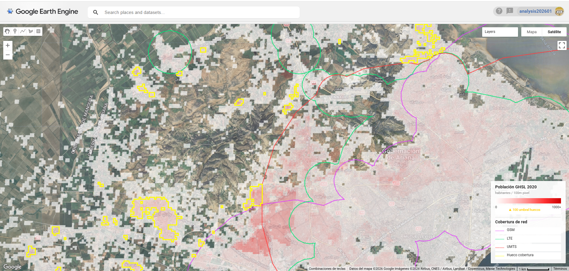
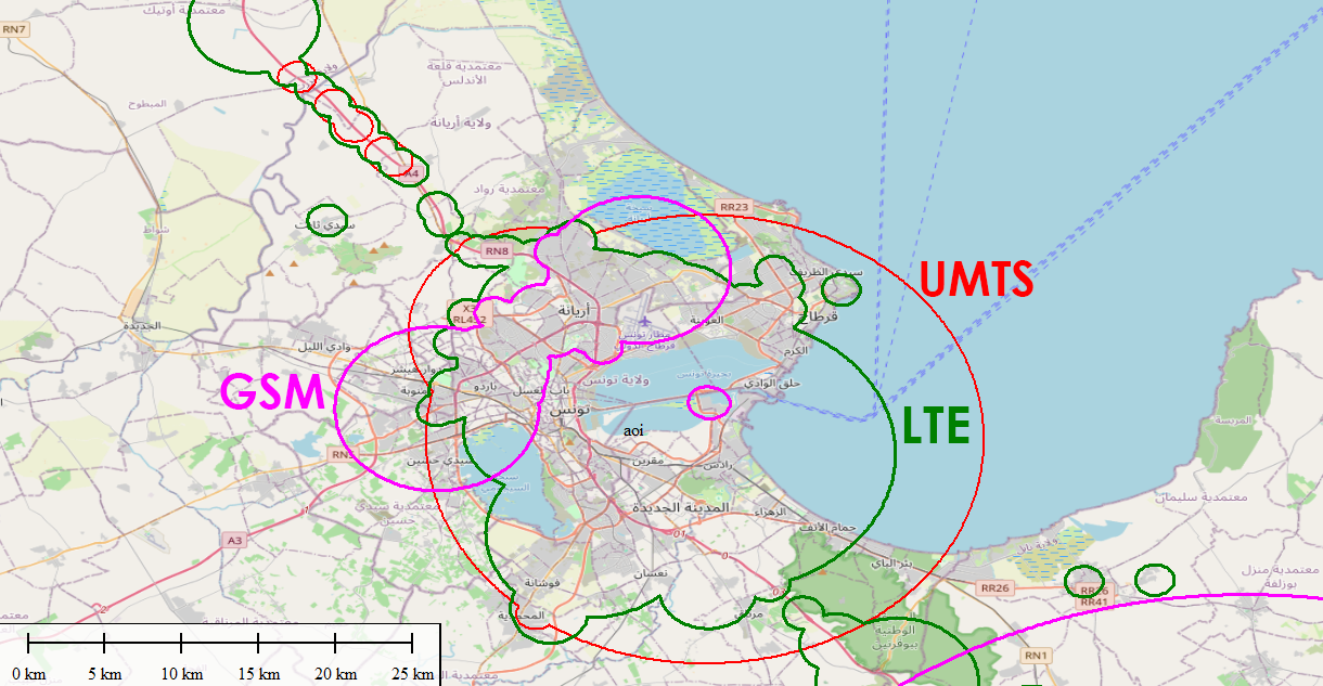
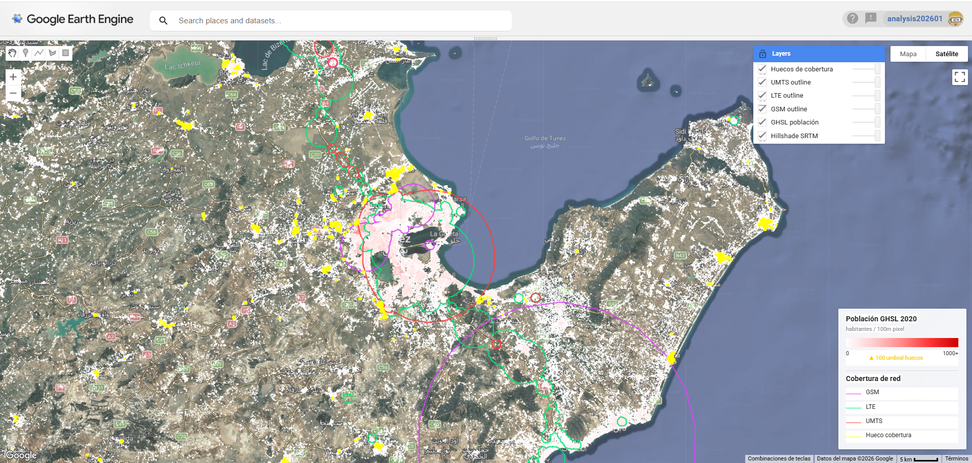
Two study areas were selected to illustrate different territorial and infrastructural conditions: Tunis and Luxembourg. Tunis represents a dense and rapidly expanding metropolitan environment with heterogeneous infrastructure distribution, while Luxembourg provides an example of a smaller and highly connected European territory with dense transport and telecommunications networks. Preliminary results show strong LTE and UMTS concentration around urban cores and major transport corridors, whereas fragmented or sparse coverage appears more frequently in peripheral settlements and lower-density areas. Several populated clusters identified through GHSL remain outside the simplified coverage envelopes, highlighting potential candidates for further connectivity assessment.
This analysis contains important limitations. OpenCellID is a crowdsourced dataset with variable completeness across regions, and the reported cell ranges are only approximate estimates rather than engineering measurements. The simplified buffering methodology does not account for terrain effects, signal attenuation, antenna directionality or radio interference, while GHSL population values are themselves modeled estimates. Consequently, the results should be interpreted as exploratory indicators of possible connectivity gaps rather than authoritative coverage maps. Nevertheless, the integration of open telecom observations, global population datasets and large-scale vector mapping frameworks demonstrates the growing potential of open geospatial ecosystems for large-scale infrastructure and digital accessibility analysis.
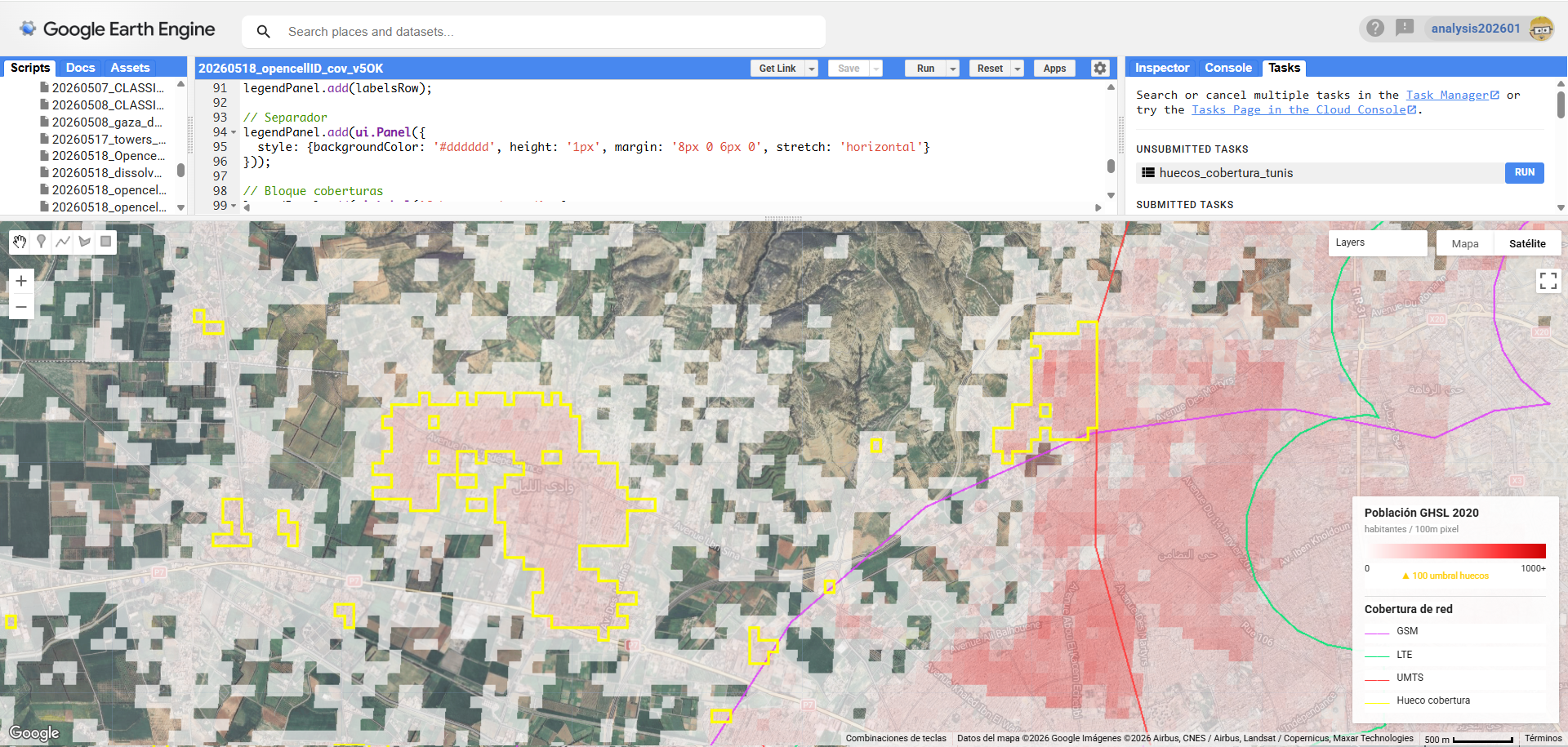
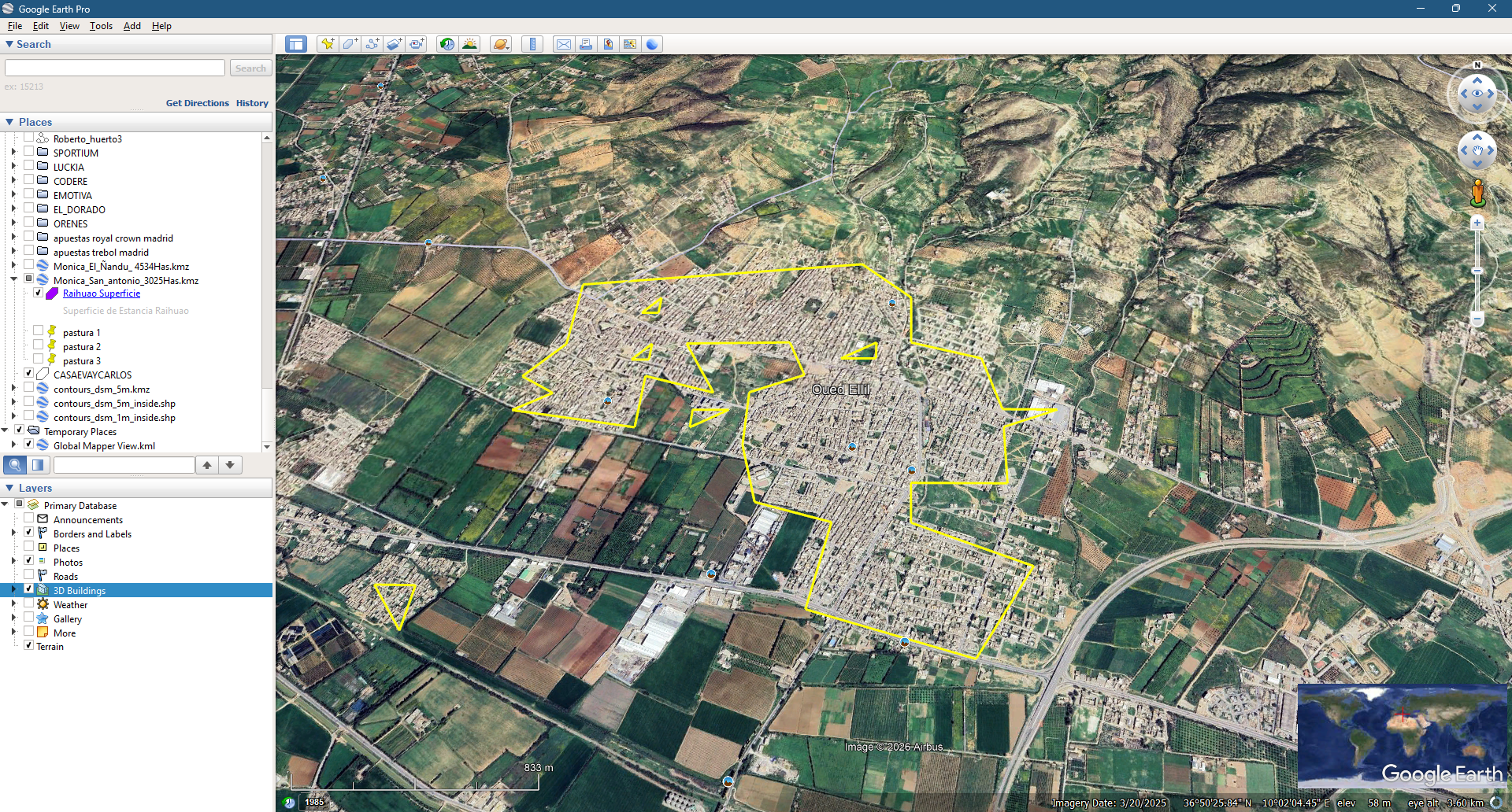
The final output of the workflow is a vector geometry representing areas where population and built-up structures exist but where no nearby cellular coverage has been identified from the technologies available in OpenCellID. These geometries can be exported and directly visualized in platforms such as Google Earth, where they highlight zones that potentially should have mobile coverage but appear to lack it according to the observed GSM, UMTS, LTE and NR datasets used in this analysis.
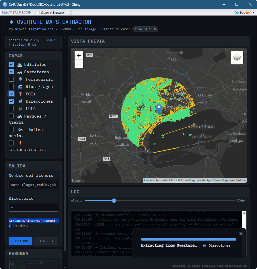
As I had introduced before, additional contextual information from Overture Maps can also be integrated into the same output, including addresses, points of interest, buildings, roads, railways, hydrography, land use and other infrastructure layers, providing a richer spatial framework to interpret the detected gaps. This entire data extraction and integration process can be reproduced in minutes using the R-based application I developed last week, which automates the retrieval and preprocessing of Overture Maps vector datasets for geospatial analysis workflows.
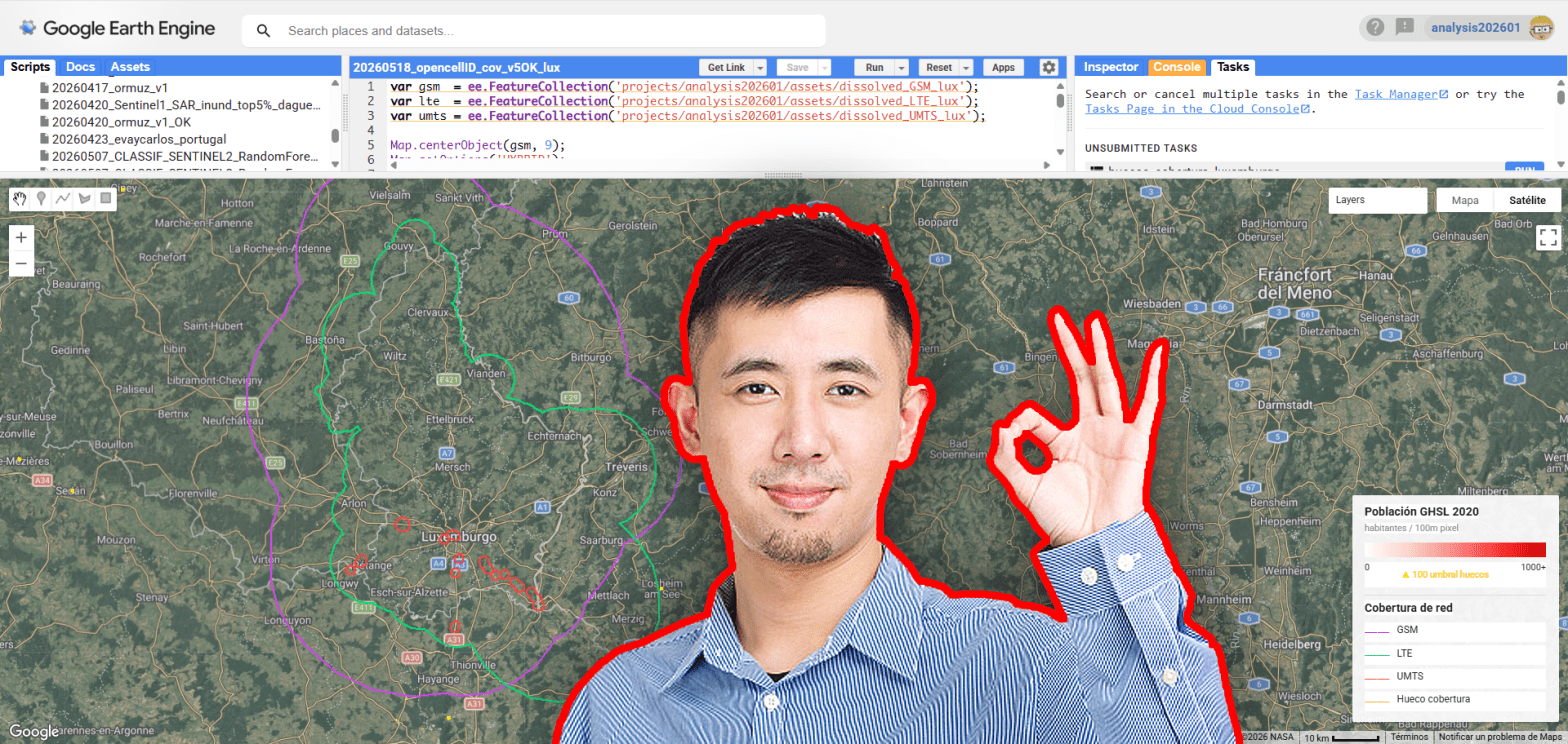
Now we can automatize the whole procedure switching to a different ASSET and that’d take just a few minutes to get to know if we have potential coverage issues we might address right away!. This below has been adapted to do the same over Luxembourg. Only to know these guys are completely covered!!
var gsm = ee.FeatureCollection('projects/analysis202601/assets/dissolved_GSM_lux');var lte = ee.FeatureCollection('projects/analysis202601/assets/dissolved_LTE_lux');var umts = ee.FeatureCollection('projects/analysis202601/assets/dissolved_UMTS_lux');Map.centerObject(gsm, 9);Map.setOptions('HYBRID');// ── SRTM hillshade ────────────────────────────────────────────var srtm = ee.Image('USGS/SRTMGL1_003');var hillshade = ee.Terrain.hillshade(srtm, 315, 45);Map.addLayer(hillshade, {min: 0, max: 255, opacity: 0.35}, 'Hillshade SRTM', true);// ── GHSL población ────────────────────────────────────────────var ghsl = ee.ImageCollection('JRC/GHSL/P2023A/GHS_POP') .filter(ee.Filter.date('2020-01-01', '2020-12-31')) .select('population_count') .mosaic();var POP_MIN = 0;var POP_MAX = 1000;var POP_THRESHOLD = 100;var popMask = ghsl.gt(POP_THRESHOLD);var ghslVis = {min: POP_MIN, max: POP_MAX, palette: ['ffffff', 'ffcccc', 'ff8888', 'ff3333', 'cc0000']};Map.addLayer(ghsl.updateMask(ghsl.gt(0)), ghslVis, 'GHSL población', true);// ── Coberturas outlined ───────────────────────────────────────var empty = ee.Image().byte();Map.addLayer(empty.paint({featureCollection: gsm, color: 1, width: 2}), {palette: ['e040fb'], opacity: 0.9}, 'GSM outline', true);Map.addLayer(empty.paint({featureCollection: lte, color: 1, width: 2}), {palette: ['00e676'], opacity: 0.9}, 'LTE outline', true);Map.addLayer(empty.paint({featureCollection: umts, color: 1, width: 2}), {palette: ['ff3d3d'], opacity: 0.9}, 'UMTS outline', true);// ── Huecos de cobertura ───────────────────────────────────────var allCoverage = gsm.merge(lte).merge(umts);var gapsImg = ee.Image(1).paint(allCoverage, 0).selfMask().updateMask(popMask);var roi = gsm.geometry().bounds().buffer(50000);var gapsVec = gapsImg.reduceToVectors({geometry: roi, scale: 100, maxPixels: 1e9});Map.addLayer(empty.paint({featureCollection: gapsVec, color: 1, width: 3}), {palette: ['ffff00'], opacity: 1}, 'Huecos de cobertura', true);Export.table.toDrive({ collection: gapsVec.map(function(f) { return f.setGeometry(f.geometry().simplify(200)); }), description: 'huecos_cobertura_luxemburgo', fileFormat: 'GeoJSON', folder: 'GEE_exports'});print('Total huecos:', gapsVec.size());print('GSM polígonos:', gsm.size());print('LTE polígonos:', lte.size());print('UMTS polígonos:', umts.size());// ── Leyenda ───────────────────────────────────────────────────var palette = ['ffffff', 'ffcccc', 'ff8888', 'ff3333', 'cc0000'];var colorbar = ui.Thumbnail({ image: ee.Image.pixelLonLat().select('longitude') .multiply((POP_MAX - POP_MIN) / 360.0) .add(POP_MAX / 2.0) .visualize({min: POP_MIN, max: POP_MAX, palette: palette}), params: {bbox: [-180, -5, 180, 5], dimensions: '200x16'}, style: {stretch: 'horizontal', margin: '4px 0px'}});var legendPanel = ui.Panel({ style: { position: 'bottom-right', padding: '10px 14px', backgroundColor: 'rgba(255,255,255,0.92)', width: '230px' }});legendPanel.add(ui.Label('Población GHSL 2020', { fontWeight: 'bold', fontSize: '13px', margin: '0 0 4px 0'}));legendPanel.add(ui.Label('habitantes / 100m pixel', { fontSize: '10px', color: '#888888', margin: '0 0 6px 0'}));legendPanel.add(colorbar);var labelsRow = ui.Panel({ layout: ui.Panel.Layout.flow('horizontal'), style: {stretch: 'horizontal', margin: '2px 0 0 0'}});labelsRow.add(ui.Label(String(POP_MIN), {fontSize: '10px', margin: '0'}));labelsRow.add(ui.Label('▲ ' + String(POP_THRESHOLD) + ' umbral huecos', { fontSize: '10px', color: '#ffcc00', textAlign: 'center', stretch: 'horizontal'}));labelsRow.add(ui.Label(POP_MAX + '+', {fontSize: '10px', margin: '0', textAlign: 'right'}));legendPanel.add(labelsRow);legendPanel.add(ui.Panel({ style: {backgroundColor: '#dddddd', height: '1px', margin: '8px 0 6px 0', stretch: 'horizontal'}}));legendPanel.add(ui.Label('Cobertura de red', { fontWeight: 'bold', fontSize: '13px', margin: '0 0 6px 0'}));var techs = [ {label: 'GSM', color: '#e040fb'}, {label: 'LTE', color: '#00e676'}, {label: 'UMTS', color: '#ff3d3d'}, {label: 'Hueco cobertura', color: '#ffff00'}];techs.forEach(function(t) { var row = ui.Panel({layout: ui.Panel.Layout.flow('horizontal'), style: {margin: '2px 0'}}); row.add(ui.Label('━━', {color: t.color, fontSize: '14px', margin: '0 8px 0 0'})); row.add(ui.Label(t.label, {fontSize: '11px', margin: '2px 0 0 0'})); legendPanel.add(row);});Map.add(legendPanel);

Alberto C.
GeoAI analyst
https://www.opencellid.org
https://human-settlement.emergency.copernicus.eu/
https://earthengine.google.com/
https://www.google.es/intl/es/earth/index.html
