
The USGS LiDAR Explorer, hosted via gishub.org, serves as a high-performance web gateway for interacting with the USGS 3D Elevation Program (3DEP) datasets. Developed by Qiusheng Wu, the platform leverages Cloud Optimized Point Clouds (COPC) and Entwine Point Tile (EPT) formats to enable seamless 3D visualization of massive LiDAR clouds directly in the browser without the need for local downloads.
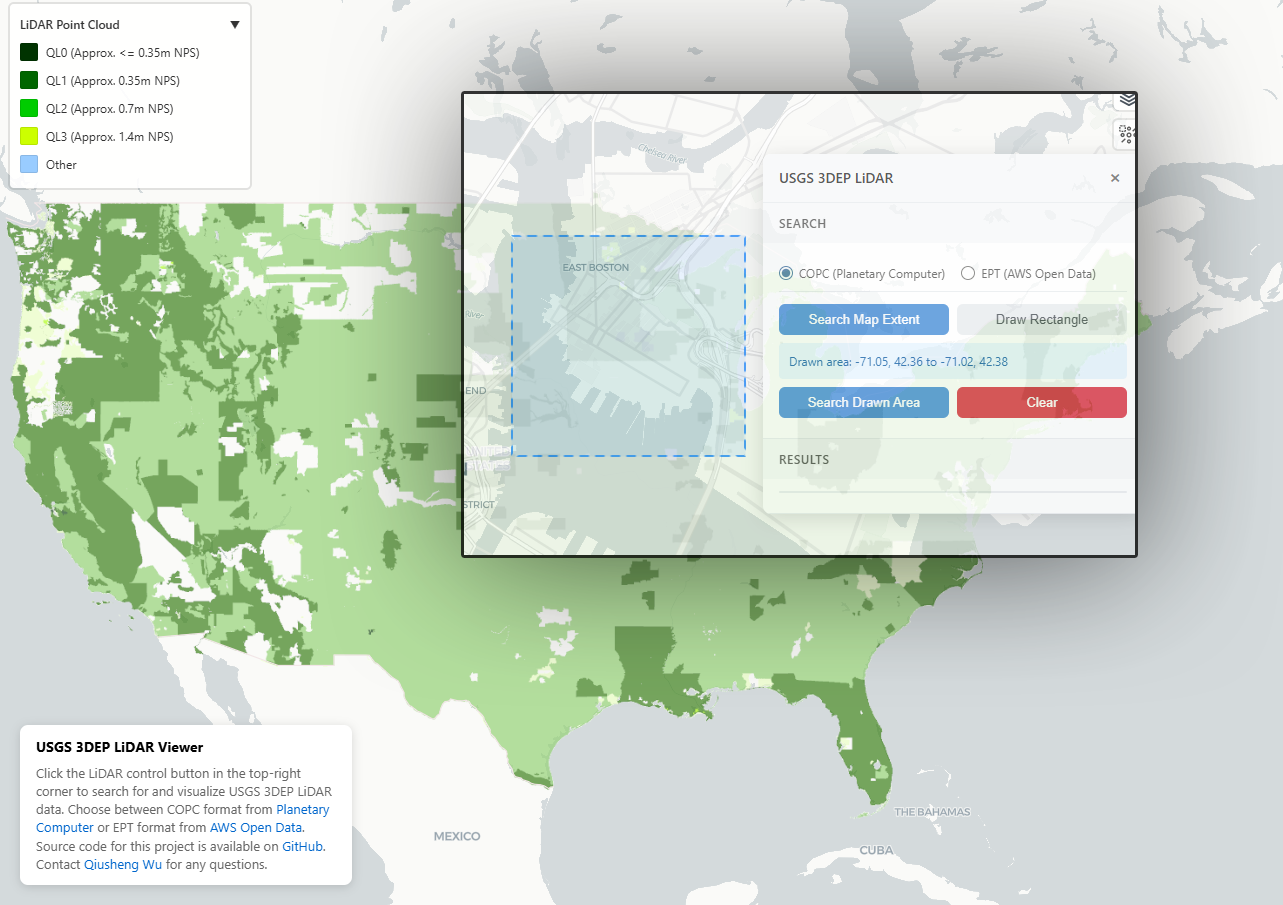
By integrating data from Microsoft Planetary Computer and AWS Open Data, it provides an essential infrastructure for researchers and developers to search, visualize, and eventually pull high-resolution elevation data into R for sophisticated urban and environmental modeling.
Now we can start playing with LIDAR! No need to download anything, just save the names of your COPCs and you can put R to work right away.
First thing, go to this GITHUB repository https://github.com/opengeos/maplibre-gl-usgs-lidar, download code for the project (code>download ZIP), get connected with RStudio, save new project and open a script window… It’s all set up!
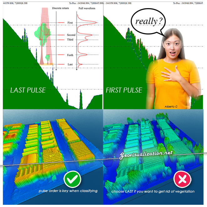
Cloud Optimized Point Clouds (COPC) represent a modernization of the standard LAZ format, specifically designed to handle massive LiDAR datasets within cloud-native environments. By reorganizing the data into a clustered octree structure, COPC allows software to stream only the specific portions or levels of detail needed for a task without downloading the entire file. This efficiency makes it the backbone of platforms like the USGS LiDAR Explorer, enabling high-speed 3D visualization and analysis directly from remote servers while maintaining full backward compatibility with traditional LAS/LAZ readers.
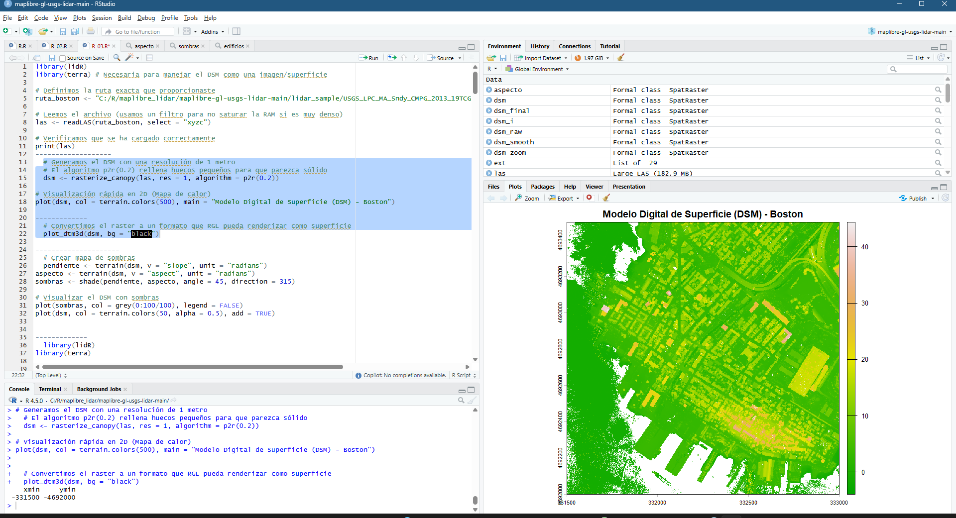
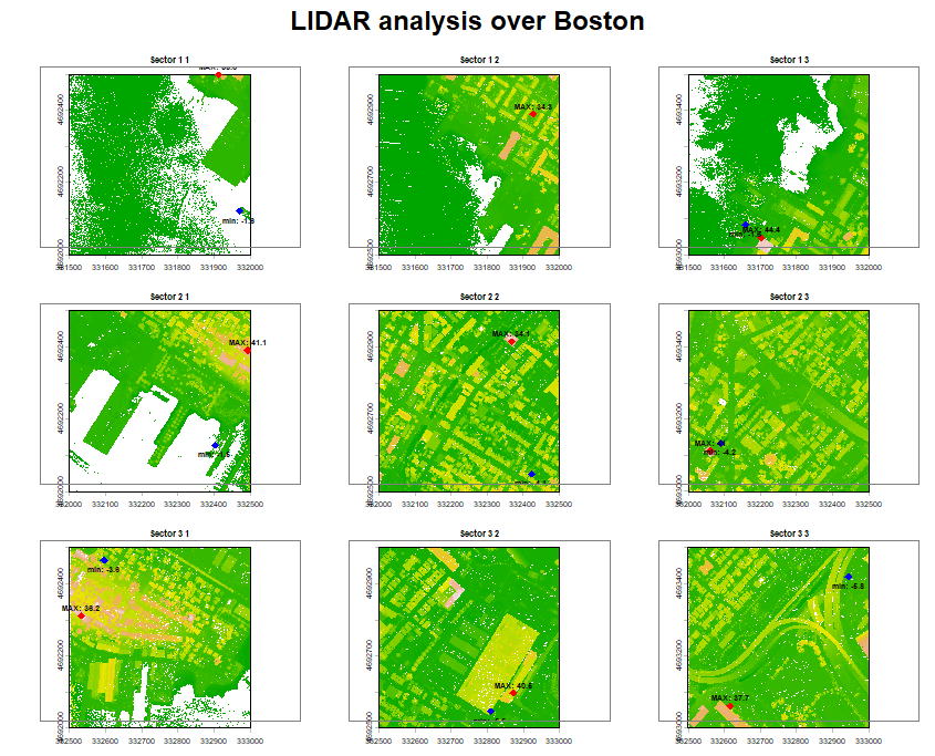
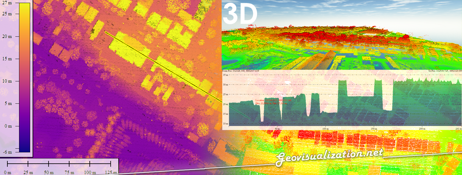
library(lidR)library(terra) # Necesaria para manejar el DSM como una imagen/superficie# Definimos la ruta exacta que proporcionasteruta_boston <- "C:/R/maplibre_lidar/maplibre-gl-usgs-lidar-main/lidar_sample/USGS_LPC_MA_Sndy_CMPG_2013_19TCG315920_LAS_2015.copc.laz"# Leemos el archivo (usamos un filtro para no saturar la RAM si es muy denso)las <- readLAS(ruta_boston, select = "xyzc")# Verificamos que se ha cargado correctamenteprint(las)-------------------# Generamos el DSM con una resolución de 1 metro# El algoritmo p2r(0.2) rellena huecos pequeños para que parezca sólidodsm <- rasterize_canopy(las, res = 1, algorithm = p2r(0.2))# Visualización rápida en 2D (Mapa de calor)plot(dsm, col = terrain.colors(50), main = "Modelo Digital de Superficie (DSM) - Boston")-------------# Convertimos el raster a un formato que RGL pueda renderizar como superficieplot_dtm3d(dsm, bg = "black")---------------------# Crear mapa de sombraspendiente <- terrain(dsm, v = "slope", unit = "radians")aspecto <- terrain(dsm, v = "aspect", unit = "radians")sombras <- shade(pendiente, aspecto, angle = 45, direction = 315)# Visualizar el DSM con sombrasplot(sombras, col = grey(0:100/100), legend = FALSE)plot(dsm, col = terrain.colors(50, alpha = 0.5), add = TRUE)-------------library(lidR)library(terra)# 1. Cargar el archivo completo (Ruta que confirmaste)ruta_boston <- "C:/R/maplibre_lidar/maplibre-gl-usgs-lidar-main/lidar_sample/USGS_LPC_MA_Sndy_CMPG_2013_19TCG315920_LAS_2015.copc.laz"las <- readLAS(ruta_boston, select = "xyzc")# 2. Elegimos una zona con edificios (puedes ajustar estos números tras ver el summary)# Estos valores suelen estar en el rango del summary(las)subset_las <- clip_rectangle(las, 331500, 4691500, 331700, 4691700)# 3. Generar el DSM (Superficie sólida) de alta resolución# Usamos res = 0.5 para que el zoom se vea nítidodsm_zoom <- rasterize_canopy(subset_las, res = 0.5, algorithm = p2r(0.3))--------------------library(lidR)library(terra)# 1. Cargar el archivo de Bostonruta_boston <- "C:/R/maplibre_lidar/maplibre-gl-usgs-lidar-main/lidar_sample/USGS_LPC_MA_Sndy_CMPG_2013_19TCG315920_LAS_2015.copc.laz"las <- readLAS(ruta_boston, select = "xyzc")# 2. Selección automática de la zona central (Cubo de 160m x 160m)x_mid <- mean(c(las@header@PHB$`Max X`, las@header@PHB$`Min X`))y_mid <- mean(c(las@header@PHB$`Max Y`, las@header@PHB$`Min Y`))subset_las <- clip_rectangle(las, x_mid - 80, y_mid - 80, x_mid + 80, y_mid + 80)# 3. Crear el DSM (Superficie continua)# El parámetro p2r(0.3) rellena los espacios vacíos entre rebotes del láserdsm_final <- rasterize_canopy(subset_las, res = 0.5, algorithm = p2r(0.3))# 4. Visualización 3D Sólidaplot_dtm3d(dsm_final, bg = "black", col = "lightblue")--------------install.packages("viridis")--------------------library(lidR)library(terra)library(viridis) # Ahora que ya está instalado# 1. Aseguramos que la superficie esté bien calculada# Usamos un radio de 0.4 para cerrar huecos sin crear "picos"dsm_raw <- rasterize_canopy(subset_las, res = 0.5, algorithm = p2r(0.4))# 2. Suavizado (El secreto de la visualización NEAT)# Aplicamos un filtro de media para que los techos se vean planos y lisosdsm_smooth <- focal(dsm_raw, w = matrix(1, 3, 3), fun = mean, na.rm = TRUE)# 3. Renderizado 3D Estilo Maqueta# 'border = NA' elimina las líneas negras que ensucian la imagen# 'col = viridis(256)' aplica el degradado profesionalplot_dtm3d(dsm_smooth, bg = "black", col = viridis(256), border = NA, lighting = TRUE)---------------- plot_dtm3d(dsm_smooth, bg = "white", col = "grey90", border = NA, lighting = TRUE)-----------------install.packages("magick")library(magick)-----------------library(rgl)# 1. Asegúrate de que la ventana de RGL esté abierta con tu modelo# 2. Definimos la función de giro (alrededor del eje Z)girar_camara <- spin3d(axis = c(0, 0, 1), rpm = 3) # 3 revoluciones por minuto# 3. Grabar la animación# Esto creará un archivo llamado "boston_360_02.gif" en tu carpeta de trabajomovie3d( f = girar_camara, duration = 20, # Duración en segundos dir = getwd(), # Se guarda donde tengas el proyecto movie = "boston_360_02", type = "gif", clean = TRUE # Borra los fotogramas sueltos al terminar)----------------------play3d(spin3d(axis = c(0, 0, 1), rpm = 10), duration = 10)---------------------movie3d( f = spin3d(axis = c(0, 0, 1), rpm = 3), duration = 10, dir = getwd(), movie = "boston_360_03", type = "gif", clean = TRUE)------------------- # Guarda la vista actual como una imagen PNG nítida snapshot3d("Boston_Maqueta_Pro.png", fmt = "png", width = 1200, height = 900)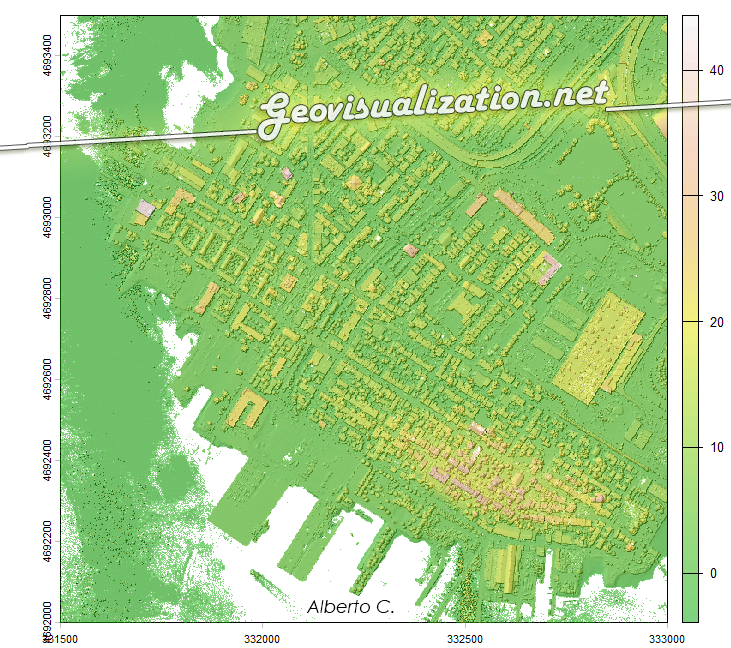
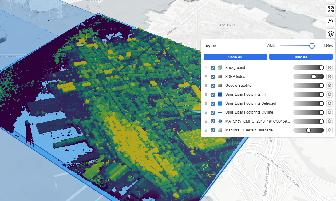
Integrating LiDAR with Open Data in R transforms your POINTS into decisions by fusing i.e physical geometry (OSMs) with precise height (LIDARs), roof pitch, and volume of every structure in a neighborhood, which is essential for determining solar energy potential or tax assessments without manual surveys.
Beyond architecture, this workflow excels in environmental management when you link city-managed tree inventories with point cloud segments. By isolating individual tree crowns in the LiDAR data and joining them to open databases via their geographic coordinates, R can report on the specific health, biomass, and carbon capture of different species across the city. You can also derive micro-topography from a LiDAR ground model and intersect it with open hydrography or sewage network data to simulate precise flood pathways during extreme weather, predicting exactly which street corners will flood based on the actual height of the curbs and pavement.
It’s a lot what you can do integrating different technologies and different kind of data…
Do you want me to surf your LIDAR dataset and extract, classify, integrate, merge or challenge it with other data? Let’s talk. I’m free and easy:-) and the most important, looking for interesting projects, well, a job:-)
Alberto C.
Geodata analyst
Sources:
https://github.com/opengeos/maplibre-gl-usgs-lidar
https://usgs-lidar.gishub.org/
