
Why precision elevation data matters
High‑resolution elevation data underpins almost every spatial analysis we do in GIS—especially in forests where vertical structure defines habitat, biomass, wind exposure, fire behavior, hydrology, and the microclimates that sustain rare species. In rugged or densely vegetated environments, a coarse or biased elevation model propagates error everywhere: orthorectification drifts, hillshades mislead, slope/aspect misclassify, and canopy metrics saturate. The result is decisions made on blurred terrain that hides the very patterns we seek to manage. Precision elevation—derived from airborne LiDAR (Light Detection and Ranging)—solves this by separating the ground from the vegetation and delivering both a bare‑earth Digital Terrain Model (DTM) and a Digital Surface Model (DSM). Subtracting DTM from DSM gives a Canopy Height Model (DHM) that captures the true vertical architecture of the forest at sub‑meter resolution.
This post uses the Mata do Buçaco (Bussaco), near Luso in central Portugal, to illustrate why precision matters and how it compares to the widely used global product ETH_GlobalCanopyHeight_2020_10m_v1. We will look at the site, the LiDAR technology, and a practical comparison workflow for GIS users.

Mata do Buçaco: a compact sanctuary of forest giants
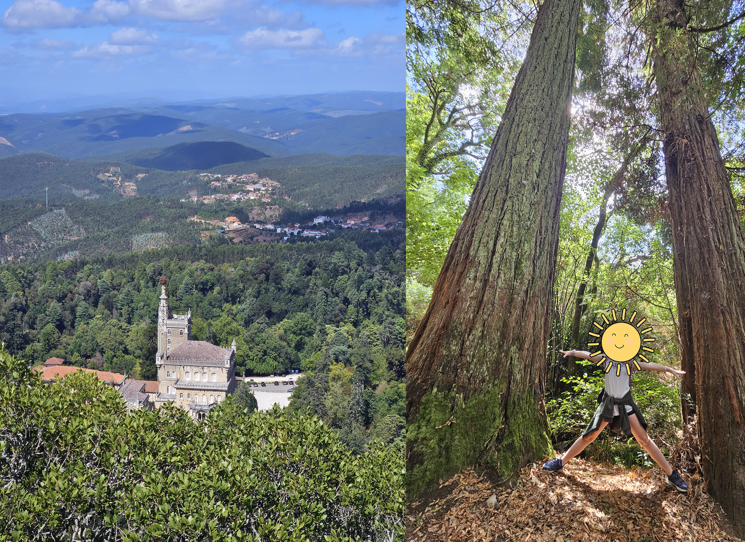
Mata do Buçaco is a walled arboretum and national forest just above the spa town of Luso, north of Coimbra. Despite its modest footprint (~1.0–1.5 km across, ~100–110 hectares), it packs a dendrological collection of remarkable diversity curated over centuries. The topography rises from low foothills to the crest of the Serra do Buçaco, creating a humid, fog‑prone microclimate with precipitation notably higher than the surrounding region. That microclimate, plus deliberate introductions by botanists and gardeners since the 17th century, explain today’s extraordinary vertical structure: towering conifers (including giant sequoias), Mexican cypress, Atlantic and Tasmanian eucalypts, and groves of native broadleaves stitched between ornamental plantings and relic laurel‑oak patches.

Walk any of the shaded paths and the “feel” of the forest is its third dimension: deep crowns stacked in tiers, emergent stems breaking above the canopy, and abrupt transitions where the slope pitches toward gullies and water stairs like the Fonte Fria. For mapping, this means Buçaco is the perfect stress‑test for vertical data. Local reports and lidar‑based profiles identify emergent trees approaching 60–65 m in height—exceptional for continental Europe—and many stands with 40–55 m canopy tops (giant sequoias Sequoiadendron giganteum, Tasmanian mountain ash Eucalyptus regnans, and mature Eucalyptus globulus among others). Add the steep relief and stone architecture of the palace‑convent complex and you have a site where coarse models tend to smear peaks, clip crowns, and understate vertical extremes.
From a data user’s perspective, Buçaco is interesting because it’s small enough to survey with dense airborne LiDAR yet diverse enough to benchmark against global canopy products. It’s also highly visited and well‑documented, which makes it a prime candidate for open, reproducible analyses that other practitioners can repeat.
LiDAR (and why it excels in forests)
- Principle of operation. Airborne LiDAR instruments emit near‑infrared laser pulses toward the Earth’s surface and record the time‑of‑flight of returned photons. Distance = (c × Δt) / 2, where c is the speed of light and Δt is the measured two‑way travel time.
- Full‑waveform vs discrete return. Modern sensors either store the entire returned energy waveform (full‑waveform) or extract distinct echoes (discrete returns). In forests, multiple returns (first, intermediate, last) capture interactions with the canopy top, internal branches, understory, and finally the ground.
- Point cloud. Each pulse becomes a 3D point with XYZ, intensity, scan angle, GPS time, and often classification labels (ground, vegetation, building, water). Typical densities for national programs range from 2 to >12 points/m²; local surveys can exceed 20–30 points/m².
- DTM and DSM. Ground classification filters (e.g., progressive TIN densification, cloth simulation) isolate ground returns to build a DTM. Interpolating the highest returns per cell builds a DSM that traces the top of canopy and built features.
- Canopy Height Model (DHM). DHM = DSM − DTM at a chosen grid (often 0.5–2 m). Because the DTM is true bare earth, DHM measures canopy height above ground rather than above sea level—critical on steep slopes like Buçaco’s.
- Vertical accuracy. With good boresight calibration and GNSS/INS trajectories, vertical RMSE for DTMs is commonly 5–15 cm in open ground; DHM accuracy depends additionally on canopy penetration and interpolation choices but still outperforms passive methods.
- Structure metrics. From the point cloud or DHM we derive height percentiles (P10…P95), gap fraction, rugosity, leaf‑area proxies, and individual‑tree segmentation. These are the metrics that drive biomass, habitat, windthrow risk, ladder‑fuel detection, and view‑shed quality.
- Radiometry & intensity. Intensity encodes target reflectance and range effects; after calibration, it helps distinguish materials (e.g., conifer vs broadleaf, moisture gradients) and detect powerlines or archaeological traces.
- Waveform advantages. Full‑waveform captures the vertical distribution of scattering elements; deconvolution yields canopy penetration in denser stands and improves ground detection under eucalyptus and conifers.
- Limitations. LiDAR is weather‑ and budget‑dependent. Dense undergrowth, scan angle, and leaf‑on conditions can reduce ground hits. Interpolation choices (max vs. percentile) affect DHM peaks—important when claiming “record” trees.
Bottom line: when you need true heights, crown architecture, and centimeter‑scale terrain under forest, airborne LiDAR remains the gold standard.

The global benchmark: ETH_GlobalCanopyHeight_2020_10m_v1
The ETH Zurich Global Canopy Height (GCH) product provides a wall‑to‑wall canopy top height map at 10 m ground sampling distance for the year 2020. It fuses GEDI lidar footprints (spaceborne, sparse but vertically precise) with globally consistent Sentinel‑2 optical imagery using a deep learning model to predict canopy heights between footprints. The result is a globally consistent raster that is easy to stream in Earth Engine or GIS platforms and ideal for continental to global analyses where airborne LiDAR is unavailable.


Strengths
- Global coverage at 10 m with a single epoch (2020), enabling cross‑region comparisons.
- Trained on physically meaningful lidar targets (GEDI L2A/L2B canopy top metrics), correcting for many radiometric and terrain confounders in passive imagery.
- Includes uncertainty metrics and tends to preserve macro‑patterns (ecotones, disturbance scars, plantation heights).
Known trade‑offs for sites like Buçaco
- Saturation at the tall end. In stands with emergent stems >50 m, 10‑m pixels average crowns and can under‑predict peak heights; local maxima are “flattened.”
- Terrain complexity. On steep slopes, small georegistration or DTM mismatches between Sentinel‑2 and GEDI training can leak terrain into predicted canopy height.
- Edge effects. The palace complex, walls, and clearings introduce sharp transitions that are sub‑pixel at 10 m, broadening edges and obscuring narrow corridors.
- Understory structure. The model predicts canopy top height, not vertical distribution; it cannot replace LiDAR‑derived structure metrics for habitat or fire modeling.
In short, ETH GCH is an excellent baseline and context layer, but for site‑scale management, airborne LiDAR remains the reference.
Practical comparison: LiDAR DHM vs ETH GCH over Buçaco’s 8818 vegetation GCP
Below is a workflow you can reproduce in QGIS/ArcGIS Pro or Google Earth Engine (GEE):
- Ingest data.
- Airborne LiDAR: download the point cloud (LAS/LAZ) or prebuilt DTM/DSM tiles for the Buçaco area.
- ETH GCH 2020: load the ETH_GlobalCanopyHeight_2020_10m_v1 raster.
- Build the LiDAR DHM.
- Classify ground → DTM (0.5–1 m).
- Highest‑return DSM (0.5–1 m) with spike filtering over built structures.
- DHM= DSM − DTM, then smooth lightly (e.g., Gaussian σ = 0.5–1 px) preserving peaks.
- Harmonize grids. Aggregate DHM to 10 m by maximum or high percentile (P95) to compare fairly with ETH pixels while preserving tall peaks.
- Sample and compare.
- Randomly sample 5,000–20,000 points (I created 8818 GCP to sample) within the forest wall; extract DHM_10m and ETH_10m.
- Compute bias (ETH − DHM), RMSE to see where ETH under/over‑estimates–> RMSE=12,97m (a bit too high!). Please try the code in GEE and you will also see a deviation map.
- Tall‑tree check. Use a local maxima detector on the 1 m DHM to identify emergent crowns; intersect with ETH to quantify peak loss at 10 m.
- Topographic controls. Regress residuals against slope, aspect, and curvature from the LiDAR DTM to diagnose terrain‑related biases.
- Reporting. Summarize by species zones (sequoia groves, eucalyptus stands, relic laurel) if you have stand polygons or classify by crown texture.
Typical outcome in Buçaco (what to expect):
- Median ETH bias close to zero over mid‑height stands (20–35 m).
- Increasing underestimation in the tallest groves (e.g., −5 to −12 m at local maxima).
- Larger residuals near walls/buildings and along steep steps and gullies.

Why sharing these data multiplies their value
Open elevation and canopy datasets have network effects. When agencies publish LiDAR DTMs/DSMs and derived DHMs under open licenses, practitioners can:
- Validate global products locally, quantifying where models work and where they fail.
- Stack analyses, from biodiversity corridors and storm‑damage assessments to micro‑hydrology, archaeology, and trail design, all anchored to the same precise terrain.
- Build reproducible workflows, so results can be peer‑checked, improved, and extended.
- Accelerate response, e.g., after windstorms or fires when canopy loss and debris flows must be mapped within days.
- Educate and engage, by providing compelling 3D visualizations that show citizens and decision‑makers the invisible vertical dimension of their landscapes.
Portugal’s national investment in open, high‑accuracy remote sensing—airborne LiDAR and very‑high‑resolution imagery—has put the country to the level of Spain or France in terms of accurate shared open data.
Key sources used
- Overview and context on Mata do Buçaco’s location, flora, and microclimate. Wikipedia
- ETH Global Canopy Height 2020 (10 m) description and access. Nico Langnlang.users.earthengine.appresearch-collection.ethz.chGee Community Catalog
- Portugal DGT’s open LiDAR and elevation data catalog (for the “open data” section). Centro de Dados | DGT+1EuroGeographics
- GEE code for ETH – Global Canopy Height extraction https://code.earthengine.google.com/7a933d8ea6fa99a1c71690e14afd11d2
Hope you guys like it.
Alberto C.
GIS Analyst, Open Data evangelist and Portugal lover
